63 OLS Goodness of Fit
63.1 Pythagorean Theorem
PythMod
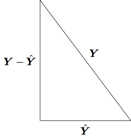
Least squares model fitting can be understood through the Pythagorean theorem: \(a^2 + b^2 = c^2\). However, here we have:
\[ \sum_{i=1}^n Y_i^2 = \sum_{i=1}^n \hat{Y}_i^2 + \sum_{i=1}^n (Y_i - \hat{Y}_i)^2 \]
where the \(\hat{Y}_i\) are the result of a linear projection of the \(Y_i\).
63.2 OLS Normal Model
In this section, let’s assume that \(({\boldsymbol{X}}_1, Y_1), \ldots, ({\boldsymbol{X}}_n, Y_n)\) are distributed so that
\[ \begin{aligned} Y_i & = \beta_1 X_{i1} + \beta_2 X_{i2} + \ldots + \beta_p X_{ip} + E_i \\ & = {\boldsymbol{X}}_i {\boldsymbol{\beta}}+ E_i \end{aligned} \]
where \({\boldsymbol{E}}| {\boldsymbol{X}}\sim \mbox{MVN}_n({\boldsymbol{0}}, \sigma^2 {\boldsymbol{I}})\). Note that we haven’t specified the distribution of the \({\boldsymbol{X}}_i\) rv’s.
63.3 Projection Matrices
In the OLS framework we have:
\[ \hat{{\boldsymbol{Y}}} = {\boldsymbol{X}}({\boldsymbol{X}}^T {\boldsymbol{X}})^{-1} {\boldsymbol{X}}^T {\boldsymbol{Y}}. \]
The matrix \({\boldsymbol{P}}_{n \times n} = {\boldsymbol{X}}({\boldsymbol{X}}^T {\boldsymbol{X}})^{-1} {\boldsymbol{X}}^T\) is a projection matrix. The vector \({\boldsymbol{Y}}\) is projected into the space spanned by the column space of \({\boldsymbol{X}}\).
Project matrices have the following properties:
- \({\boldsymbol{P}}\) is symmetric
- \({\boldsymbol{P}}\) is idempotent so that \({\boldsymbol{P}}{\boldsymbol{P}}= {\boldsymbol{P}}\)
- If \({\boldsymbol{X}}\) has column rank \(p\), then \({\boldsymbol{P}}\) has rank \(p\)
- The eigenvalues of \({\boldsymbol{P}}\) are \(p\) 1’s and \(n-p\) 0’s
- The trace (sum of diagonal entries) is \(\operatorname{tr}({\boldsymbol{P}}) = p\)
- \({\boldsymbol{I}}- {\boldsymbol{P}}\) is also a projection matrix with rank \(n-p\)
63.4 Decomposition
Note that \({\boldsymbol{P}}({\boldsymbol{I}}- {\boldsymbol{P}}) = {\boldsymbol{P}}- {\boldsymbol{P}}{\boldsymbol{P}}= {\boldsymbol{P}}- {\boldsymbol{P}}= {\boldsymbol{0}}\).
We have
\[ \begin{aligned} \| {\boldsymbol{Y}}\|_{2}^{2} = {\boldsymbol{Y}}^T {\boldsymbol{Y}}& = ({\boldsymbol{P}}{\boldsymbol{Y}}+ ({\boldsymbol{I}}- {\boldsymbol{P}}) {\boldsymbol{Y}})^T ({\boldsymbol{P}}{\boldsymbol{Y}}+ ({\boldsymbol{I}}- {\boldsymbol{P}}) {\boldsymbol{Y}}) \\ & = ({\boldsymbol{P}}{\boldsymbol{Y}})^T ({\boldsymbol{P}}{\boldsymbol{Y}}) + (({\boldsymbol{I}}- {\boldsymbol{P}}) {\boldsymbol{Y}})^T (({\boldsymbol{I}}- {\boldsymbol{P}}) {\boldsymbol{Y}}) \\ & = \| {\boldsymbol{P}}{\boldsymbol{Y}}\|_{2}^{2} + \| ({\boldsymbol{I}}- {\boldsymbol{P}}) {\boldsymbol{Y}}\|_{2}^{2} \end{aligned} \]
where the cross terms disappear because \({\boldsymbol{P}}({\boldsymbol{I}}- {\boldsymbol{P}}) = {\boldsymbol{0}}\).
Note: The \(\ell_p\) norm of an \(n\)-vector \(\boldsymbol{w}\) is defined as
\[ \| \boldsymbol{w} \|_p = \left(\sum_{i=1}^n |w_i|^p\right)^{1/p}. \]
Above we calculated
\[ \| \boldsymbol{w} \|_2^2 = \sum_{i=1}^n w_i^2. \]
63.5 Distribution of Projection
Suppose that \(Y_1, Y_2, \ldots, Y_n {\; \stackrel{\text{iid}}{\sim}\;}\mbox{Normal}(0,\sigma^2)\). This can also be written as \({\boldsymbol{Y}}\sim \mbox{MVN}_n({\boldsymbol{0}}, \sigma^2 {\boldsymbol{I}})\). It follows that
\[ {\boldsymbol{P}}{\boldsymbol{Y}}\sim \mbox{MVN}_{n}({\boldsymbol{0}}, \sigma^2 {\boldsymbol{P}}{\boldsymbol{I}}{\boldsymbol{P}}^T). \]
where \({\boldsymbol{P}}{\boldsymbol{I}}{\boldsymbol{P}}^T = {\boldsymbol{P}}{\boldsymbol{P}}^T = {\boldsymbol{P}}{\boldsymbol{P}}= {\boldsymbol{P}}\).
Also, \(({\boldsymbol{P}}{\boldsymbol{Y}})^T ({\boldsymbol{P}}{\boldsymbol{Y}}) = {\boldsymbol{Y}}^T {\boldsymbol{P}}^T {\boldsymbol{P}}{\boldsymbol{Y}}= {\boldsymbol{Y}}^T {\boldsymbol{P}}{\boldsymbol{Y}}\), a quadratic form. Given the eigenvalues of \({\boldsymbol{P}}\), \({\boldsymbol{Y}}^T {\boldsymbol{P}}{\boldsymbol{Y}}\) is equivalent in distribution to \(p\) squared iid Normal(0,1) rv’s, so
\[ \frac{{\boldsymbol{Y}}^T {\boldsymbol{P}}{\boldsymbol{Y}}}{\sigma^2} \sim \chi^2_{p}. \]
63.6 Distribution of Residuals
If \({\boldsymbol{P}}{\boldsymbol{Y}}= \hat{{\boldsymbol{Y}}}\) are the fitted OLS values, then \(({\boldsymbol{I}}-{\boldsymbol{P}}) {\boldsymbol{Y}}= {\boldsymbol{Y}}- \hat{{\boldsymbol{Y}}}\) are the residuals.
It follows by the same argument as above that
\[ \frac{{\boldsymbol{Y}}^T ({\boldsymbol{I}}-{\boldsymbol{P}}) {\boldsymbol{Y}}}{\sigma^2} \sim \chi^2_{n-p}. \]
It’s also straightforward to show that \(({\boldsymbol{I}}-{\boldsymbol{P}}){\boldsymbol{Y}}\sim \mbox{MVN}_{n}({\boldsymbol{0}}, \sigma^2({\boldsymbol{I}}-{\boldsymbol{P}}))\) and \({\operatorname{Cov}}({\boldsymbol{P}}{\boldsymbol{Y}}, ({\boldsymbol{I}}-{\boldsymbol{P}}){\boldsymbol{Y}}) = {\boldsymbol{0}}\).
63.7 Degrees of Freedom
The degrees of freedom, \(p\), of a linear projection model fit is equal to
- The number of linearly independent columns of \({\boldsymbol{X}}\)
- The number of nonzero eigenvalues of \({\boldsymbol{P}}\) (where nonzero eigenvalues are equal to 1)
- The trace of the projection matrix, \(\operatorname{tr}({\boldsymbol{P}})\).
The reason why we divide estimates of variance by \(n-p\) is because this is the number of effective independent sources of variation remaining after the model is fit by projecting the \(n\) observations into a \(p\) dimensional linear space.
63.8 Submodels
Consider the OLS model \({\boldsymbol{Y}}= {\boldsymbol{X}}{\boldsymbol{\beta}}+ {\boldsymbol{E}}\) where there are \(p\) columns of \({\boldsymbol{X}}\) and \({\boldsymbol{\beta}}\) is a \(p\)-vector.
Let \({\boldsymbol{X}}_0\) be a subset of \(p_0\) columns of \({\boldsymbol{X}}\) and let \({\boldsymbol{X}}_1\) be a subset of \(p_1\) columns, where \(1 \leq p_0 < p_1 \leq p\). Also, assume that the columns of \({\boldsymbol{X}}_0\) are a subset of \({\boldsymbol{X}}_1\).
We can form \(\hat{{\boldsymbol{Y}}}_0 = {\boldsymbol{P}}_0 {\boldsymbol{Y}}\) where \({\boldsymbol{P}}_0\) is the projection matrix built from \({\boldsymbol{X}}_0\). We can analogously form \(\hat{{\boldsymbol{Y}}}_1 = {\boldsymbol{P}}_1 {\boldsymbol{Y}}\).
63.9 Hypothesis Testing
Without loss of generality, suppose that \({\boldsymbol{\beta}}_0 = (\beta_1, \beta_2, \ldots, \beta_{p_0})^T\) and \({\boldsymbol{\beta}}_1 = (\beta_1, \beta_2, \ldots, \beta_{p_1})^T\).
How do we compare these models, specifically to test \(H_0: (\beta_{p_0+1}, \beta_{p_0 + 2}, \ldots, \beta_{p_1}) = {\boldsymbol{0}}\) vs \(H_1: (\beta_{p_0+1}, \beta_{p_0 + 2}, \ldots, \beta_{p_1}) \not= {\boldsymbol{0}}\)?
The basic idea to perform this test is to compare the goodness of fits of each model via a pivotal statistic. We will discuss the generalized LRT and ANOVA approaches.
63.10 Generalized LRT
Under the OLS Normal model, it follows that \(\hat{{\boldsymbol{\beta}}}_0 = ({\boldsymbol{X}}^T_0 {\boldsymbol{X}}_0)^{-1} {\boldsymbol{X}}_0^T {\boldsymbol{Y}}\) is the MLE under the null hypothesis and \(\hat{{\boldsymbol{\beta}}}_1 = ({\boldsymbol{X}}^T_1 {\boldsymbol{X}}_1)^{-1} {\boldsymbol{X}}_1^T {\boldsymbol{Y}}\) is the unconstrained MLE. Also, the respective MLEs of \(\sigma^2\) are
\[ \hat{\sigma}^2_0 = \frac{\sum_{i=1}^n (Y_i - \hat{Y}_{0,i})^2}{n} \]
\[ \hat{\sigma}^2_1 = \frac{\sum_{i=1}^n (Y_i - \hat{Y}_{1,i})^2}{n} \]
where \(\hat{{\boldsymbol{Y}}}_{0} = {\boldsymbol{X}}_0 \hat{{\boldsymbol{\beta}}}_0\) and \(\hat{{\boldsymbol{Y}}}_{1} = {\boldsymbol{X}}_1 \hat{{\boldsymbol{\beta}}}_1\).
The generalized LRT statistic is
\[ \lambda({\boldsymbol{X}}, {\boldsymbol{Y}}) = \frac{L\left(\hat{{\boldsymbol{\beta}}}_1, \hat{\sigma}^2_1; {\boldsymbol{X}}, {\boldsymbol{Y}}\right)}{L\left(\hat{{\boldsymbol{\beta}}}_0, \hat{\sigma}^2_0; {\boldsymbol{X}}, {\boldsymbol{Y}}\right)} \]
where \(2\log\lambda({\boldsymbol{X}}, {\boldsymbol{Y}})\) has a \(\chi^2_{p_1 - p_0}\) null distribution.
63.11 Nested Projections
We can apply the Pythagorean theorem we saw earlier to linear subspaces to get:
\[ \begin{aligned} \| {\boldsymbol{Y}}\|^2_2 & = \| ({\boldsymbol{I}}- {\boldsymbol{P}}_1) {\boldsymbol{Y}}\|_{2}^{2} + \| {\boldsymbol{P}}_1 {\boldsymbol{Y}}\|_{2}^{2} \\ & = \| ({\boldsymbol{I}}- {\boldsymbol{P}}_1) {\boldsymbol{Y}}\|_{2}^{2} + \| ({\boldsymbol{P}}_1 - {\boldsymbol{P}}_0) {\boldsymbol{Y}}\|_{2}^{2} + \| {\boldsymbol{P}}_0 {\boldsymbol{Y}}\|_{2}^{2} \end{aligned} \]
We can also use the Pythagorean theorem to decompose the residuals from the smaller projection \({\boldsymbol{P}}_0\):
\[ \| ({\boldsymbol{I}}- {\boldsymbol{P}}_0) {\boldsymbol{Y}}\|^2_2 = \| ({\boldsymbol{I}}- {\boldsymbol{P}}_1) {\boldsymbol{Y}}\|^2_2 + \| ({\boldsymbol{P}}_1 - {\boldsymbol{P}}_0) {\boldsymbol{Y}}\|^2_2 \]
63.12 F Statistic
The \(F\) statistic compares the improvement of goodness in fit of the larger model to that of the smaller model in terms of sums of squared residuals, and it scales this improvement by an estimate of \(\sigma^2\):
\[ \begin{aligned} F & = \frac{\left[\| ({\boldsymbol{I}}- {\boldsymbol{P}}_0) {\boldsymbol{Y}}\|^2_2 - \| ({\boldsymbol{I}}- {\boldsymbol{P}}_1) {\boldsymbol{Y}}\|^2_2\right]/(p_1 - p_0)}{\| ({\boldsymbol{I}}- {\boldsymbol{P}}_1) {\boldsymbol{Y}}\|^2_2/(n-p_1)} \\ & = \frac{\left[\sum_{i=1}^n (Y_i - \hat{Y}_{0,i})^2 - \sum_{i=1}^n (Y_i - \hat{Y}_{1,i})^2 \right]/(p_1 - p_0)}{\sum_{i=1}^n (Y_i - \hat{Y}_{1,i})^2 / (n - p_1)} \\ \end{aligned} \]
Since \(\| ({\boldsymbol{I}}- {\boldsymbol{P}}_0) {\boldsymbol{Y}}\|^2_2 - \| ({\boldsymbol{I}}- {\boldsymbol{P}}_1) {\boldsymbol{Y}}\|^2_2 = \| ({\boldsymbol{P}}_1 - {\boldsymbol{P}}_0) {\boldsymbol{Y}}\|^2_2\), we can equivalently write the \(F\) statistic as:
\[ \begin{aligned} F & = \frac{\| ({\boldsymbol{P}}_1 - {\boldsymbol{P}}_0) {\boldsymbol{Y}}\|^2_2 / (p_1 - p_0)}{\| ({\boldsymbol{I}}- {\boldsymbol{P}}_1) {\boldsymbol{Y}}\|^2_2/(n-p_1)} \\ & = \frac{\sum_{i=1}^n (\hat{Y}_{1,i} - \hat{Y}_{0,i})^2 / (p_1 - p_0)}{\sum_{i=1}^n (Y_i - \hat{Y}_{1,i})^2 / (n - p_1)} \end{aligned} \]
63.13 F Distribution
Suppose we have independent random variables \(V \sim \chi^2_a\) and \(W \sim \chi^2_b\). It follows that
\[ \frac{V/a}{W/b} \sim F_{a,b} \]
where \(F_{a,b}\) is the \(F\) distribution with \((a, b)\) degrees of freedom.
By arguments similar to those given above, we have
\[ \frac{\| ({\boldsymbol{P}}_1 - {\boldsymbol{P}}_0) {\boldsymbol{Y}}\|^2_2}{\sigma^2} \sim \chi^2_{p_1 - p_0} \]
\[ \frac{\| ({\boldsymbol{I}}- {\boldsymbol{P}}_1) {\boldsymbol{Y}}\|^2_2}{\sigma^2} \sim \chi^2_{n-p_1} \]
and these two rv’s are independent.
63.14 F Test
Suppose that the OLS model holds where \({\boldsymbol{E}}| {\boldsymbol{X}}\sim \mbox{MVN}_n({\boldsymbol{0}}, \sigma^2 {\boldsymbol{I}})\).
In order to test \(H_0: (\beta_{p_0+1}, \beta_{p_0 + 2}, \ldots, \beta_{p_1}) = {\boldsymbol{0}}\) vs \(H_1: (\beta_{p_0+1}, \beta_{p_0 + 2}, \ldots, \beta_{p_1}) \not= {\boldsymbol{0}}\), we can form the \(F\) statistic as given above, which has null distribution \(F_{p_1 - p_0, n - p_1}\). The p-value is calculated as \(\Pr(F^* \geq F)\) where \(F\) is the observed \(F\) statistic and \(F^* \sim F_{p_1 - p_0, n - p_1}\).
If the above assumption on the distribution of \({\boldsymbol{E}}| {\boldsymbol{X}}\) only approximately holds, then the \(F\) test p-value is also an approximation.
63.15 Example: Davis Data
> library("car")
> data("Davis", package="car")
Warning in data("Davis", package = "car"): data set 'Davis' not found
> htwt <- tbl_df(Davis)
> htwt[12,c(2,3)] <- htwt[12,c(3,2)]
> head(htwt)
# A tibble: 6 x 5
sex weight height repwt repht
<fct> <int> <int> <int> <int>
1 M 77 182 77 180
2 F 58 161 51 159
3 F 53 161 54 158
4 M 68 177 70 175
5 F 59 157 59 155
6 M 76 170 76 16563.16 Comparing Linear Models in R
Example: Davis Data
Suppose we are considering the three following models:
> f1 <- lm(weight ~ height, data=htwt)
> f2 <- lm(weight ~ height + sex, data=htwt)
> f3 <- lm(weight ~ height + sex + height:sex, data=htwt)
How do we determine if the additional terms in models f2 and f3 are needed?
63.17 ANOVA (Version 2)
A generalization of ANOVA exists that allows us to compare two nested models, quantifying their differences in terms of goodness of fit and performing a hypothesis test of whether this difference is statistically significant.
A model is nested within another model if their difference is simply the absence of certain terms in the smaller model.
The null hypothesis is that the additional terms have coefficients equal to zero, and the alternative hypothesis is that at least one coefficient is nonzero.
Both versions of ANOVA can be described in a single, elegant mathematical framework.
63.18 Comparing Two Models
with anova()
This provides a comparison of the improvement in fit from model f2 compared to model f1:
> anova(f1, f2)
Analysis of Variance Table

Model 1: weight ~ height
Model 2: weight ~ height + sex
  Res.Df   RSS Df Sum of Sq      F    Pr(>F)
1    198 14321
2    197 12816  1    1504.9 23.133 2.999e-06 ***
---
Signif. codes:  0 '***' 0.001 '**' 0.01 '*' 0.05 '.' 0.1 ' ' 1
63.19 When There’s a Single Variable Difference
Compare above anova(f1, f2) p-value to that for the sex term from the f2 model:
> library(broom)
> tidy(f2)
# A tibble: 3 x 5
  term        estimate std.error statistic  p.value
  <chr>          <dbl>     <dbl>     <dbl>    <dbl>
1 (Intercept)  -76.6     15.7        -4.88 2.23e- 6
2 height         0.811    0.0953      8.51 4.50e-15
3 sexM           8.23     1.71        4.81 3.00e- 6
63.20 Calculating the F-statistic
> anova(f1, f2)
Analysis of Variance Table

Model 1: weight ~ height
Model 2: weight ~ height + sex
  Res.Df   RSS Df Sum of Sq      F    Pr(>F)
1    198 14321
2    197 12816  1    1504.9 23.133 2.999e-06 ***
---
Signif. codes:  0 '***' 0.001 '**' 0.01 '*' 0.05 '.' 0.1 ' ' 1
How the F-statistic is calculated:
> n <- nrow(htwt)
> ss1 <- (n-1)*var(f1$residuals)
> ss1
[1] 14321.11
> ss2 <- (n-1)*var(f2$residuals)
> ss2
[1] 12816.18
> ((ss1 - ss2)/anova(f1, f2)$Df[2])/(ss2/f2$df.residual)
[1] 23.13253
63.21 Calculating the Generalized LRT
> anova(f1, f2, test="LRT")
Analysis of Variance Table

Model 1: weight ~ height
Model 2: weight ~ height + sex
  Res.Df   RSS Df Sum of Sq  Pr(>Chi)
1    198 14321
2    197 12816  1    1504.9 1.512e-06 ***
---
Signif. codes:  0 '***' 0.001 '**' 0.01 '*' 0.05 '.' 0.1 ' ' 1
> library(lmtest)
> lrtest(f1, f2)
Likelihood ratio test
Model 1: weight ~ height
Model 2: weight ~ height + sex
#Df LogLik Df Chisq Pr(>Chisq)
1 3 -710.9
2 4 -699.8 1 22.205 2.45e-06 ***
---
Signif. codes: 0 '***' 0.001 '**' 0.01 '*' 0.05 '.' 0.1 ' ' 1These tests produce slightly different answers because anova() adjusts for degrees of freedom when estimating the variance, whereas lrtest() is the strict generalized LRT. See here.
63.22 ANOVA on More Distant Models
We can compare models with multiple differences in terms:
> anova(f1, f3)
Analysis of Variance Table

Model 1: weight ~ height
Model 2: weight ~ height + sex + height:sex
  Res.Df   RSS Df Sum of Sq      F    Pr(>F)
1    198 14321
2    196 12567  2      1754 13.678 2.751e-06 ***
---
Signif. codes:  0 '***' 0.001 '**' 0.01 '*' 0.05 '.' 0.1 ' ' 1
63.23 Compare Multiple Models at Once
We can compare multiple models at once:
> anova(f1, f2, f3)
Analysis of Variance Table

Model 1: weight ~ height
Model 2: weight ~ height + sex
Model 3: weight ~ height + sex + height:sex
  Res.Df   RSS Df Sum of Sq       F    Pr(>F)
1    198 14321
2    197 12816  1   1504.93 23.4712 2.571e-06 ***
3    196 12567  1    249.04  3.8841   0.05015 .
---
Signif. codes:  0 '***' 0.001 '**' 0.01 '*' 0.05 '.' 0.1 ' ' 1