65 glm() Function in R
65.1 Example: Grad School Admissions
> mydata <-
+   read.csv("https://stats.idre.ucla.edu/stat/data/binary.csv")
> dim(mydata)
[1] 400   4
> head(mydata)
  admit gre  gpa rank
1     0 380 3.61    3
2     1 660 3.67    3
3     1 800 4.00    1
4     1 640 3.19    4
5     0 520 2.93    4
6     1 760 3.00    2
Data and analysis courtesy of http://www.ats.ucla.edu/stat/r/dae/logit.htm.
65.2 Explore the Data
> apply(mydata, 2, mean)
   admit      gre      gpa     rank
  0.3175 587.7000   3.3899   2.4850
> apply(mydata, 2, sd)
      admit         gre         gpa        rank
  0.4660867 115.5165364   0.3805668   0.9444602
>
> table(mydata$admit, mydata$rank)

     1  2  3  4
  0 28 97 93 55
  1 33 54 28 12
> ggplot(data=mydata) +
+ geom_boxplot(aes(x=as.factor(admit), y=gre))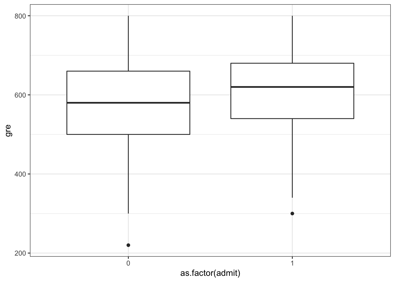
> ggplot(data=mydata) +
+   geom_boxplot(aes(x=as.factor(admit), y=gpa))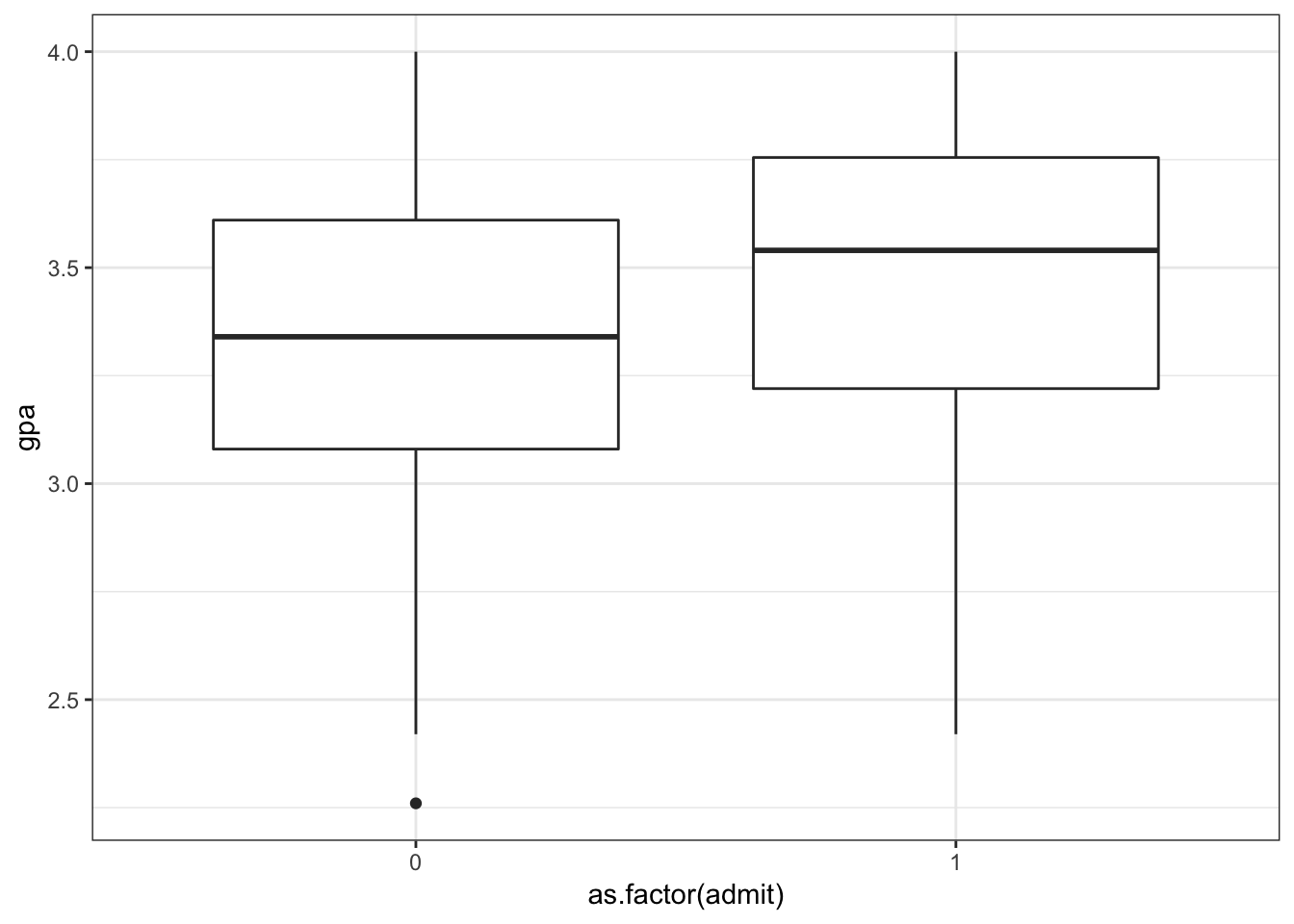
65.3 Logistic Regression in R
> mydata$rank <- factor(mydata$rank, levels=c(1, 2, 3, 4))
> myfit <- glm(admit ~ gre + gpa + rank,
+              data = mydata, family = "binomial")
> myfit

Call:  glm(formula = admit ~ gre + gpa + rank, family = "binomial",
    data = mydata)

Coefficients:
(Intercept)          gre          gpa        rank2        rank3
  -3.989979     0.002264     0.804038    -0.675443    -1.340204
      rank4
  -1.551464

Degrees of Freedom: 399 Total (i.e. Null);  394 Residual
Null Deviance:      500
Residual Deviance: 458.5    AIC: 470.5
65.4 Summary of Fit
> summary(myfit)

Call:
glm(formula = admit ~ gre + gpa + rank, family = "binomial",
    data = mydata)

Deviance Residuals:
    Min       1Q   Median       3Q      Max
-1.6268  -0.8662  -0.6388   1.1490   2.0790

Coefficients:
             Estimate Std. Error z value Pr(>|z|)
(Intercept) -3.989979   1.139951  -3.500 0.000465 ***
gre          0.002264   0.001094   2.070 0.038465 *
gpa          0.804038   0.331819   2.423 0.015388 *
rank2       -0.675443   0.316490  -2.134 0.032829 *
rank3       -1.340204   0.345306  -3.881 0.000104 ***
rank4       -1.551464   0.417832  -3.713 0.000205 ***
---
Signif. codes:  0 '***' 0.001 '**' 0.01 '*' 0.05 '.' 0.1 ' ' 1

(Dispersion parameter for binomial family taken to be 1)

    Null deviance: 499.98  on 399  degrees of freedom
Residual deviance: 458.52  on 394  degrees of freedom
AIC: 470.52

Number of Fisher Scoring iterations: 4
65.5 ANOVA of Fit
> anova(myfit, test="Chisq")
Analysis of Deviance Table

Model: binomial, link: logit

Response: admit

Terms added sequentially (first to last)

     Df Deviance Resid. Df Resid. Dev  Pr(>Chi)
NULL                   399     499.98
gre   1  13.9204       398     486.06 0.0001907 ***
gpa   1   5.7122       397     480.34 0.0168478 *
rank  3  21.8265       394     458.52 7.088e-05 ***
---
Signif. codes:  0 '***' 0.001 '**' 0.01 '*' 0.05 '.' 0.1 ' ' 1
> anova(myfit, test="LRT")
Analysis of Deviance Table

Model: binomial, link: logit

Response: admit

Terms added sequentially (first to last)

     Df Deviance Resid. Df Resid. Dev  Pr(>Chi)
NULL                   399     499.98
gre   1  13.9204       398     486.06 0.0001907 ***
gpa   1   5.7122       397     480.34 0.0168478 *
rank  3  21.8265       394     458.52 7.088e-05 ***
---
Signif. codes:  0 '***' 0.001 '**' 0.01 '*' 0.05 '.' 0.1 ' ' 1
65.6 Example: Contraceptive Use
> cuse <-
+   read.table("http://data.princeton.edu/wws509/datasets/cuse.dat",
+              header=TRUE)
> dim(cuse)
[1] 16  5
> head(cuse)
    age education wantsMore notUsing using
1   <25       low       yes       53     6
2   <25       low        no       10     4
3   <25      high       yes      212    52
4   <25      high        no       50    10
5 25-29       low       yes       60    14
6 25-29       low        no       19    10
Data and analysis courtesy of http://data.princeton.edu/R/glms.html.
65.7 A Different Format
Note that in this data set there are multiple observations per explanatory variable configuration.
The last two columns of the data frame count the successes and failures per configuration.
> head(cuse)
    age education wantsMore notUsing using
1   <25       low       yes       53     6
2   <25       low        no       10     4
3   <25      high       yes      212    52
4   <25      high        no       50    10
5 25-29       low       yes       60    14
6 25-29       low        no       19    10
65.8 Fitting the Model
When this is the case, we call the glm() function slighlty differently.
> myfit <- glm(cbind(using, notUsing) ~ age + education + wantsMore,
+              data=cuse, family = binomial)
> myfit

Call:  glm(formula = cbind(using, notUsing) ~ age + education + wantsMore,
    family = binomial, data = cuse)

Coefficients:
 (Intercept)      age25-29      age30-39      age40-49  educationlow
     -0.8082        0.3894        0.9086        1.1892       -0.3250
wantsMoreyes
     -0.8330

Degrees of Freedom: 15 Total (i.e. Null);  10 Residual
Null Deviance:      165.8
Residual Deviance: 29.92    AIC: 113.4
65.9 Summary of Fit
> summary(myfit)

Call:
glm(formula = cbind(using, notUsing) ~ age + education + wantsMore,
    family = binomial, data = cuse)

Deviance Residuals:
    Min       1Q   Median       3Q      Max
-2.5148  -0.9376   0.2408   0.9822   1.7333

Coefficients:
             Estimate Std. Error z value Pr(>|z|)
(Intercept)   -0.8082     0.1590  -5.083 3.71e-07 ***
age25-29       0.3894     0.1759   2.214  0.02681 *
age30-39       0.9086     0.1646   5.519 3.40e-08 ***
age40-49       1.1892     0.2144   5.546 2.92e-08 ***
educationlow  -0.3250     0.1240  -2.620  0.00879 **
wantsMoreyes  -0.8330     0.1175  -7.091 1.33e-12 ***
---
Signif. codes:  0 '***' 0.001 '**' 0.01 '*' 0.05 '.' 0.1 ' ' 1

(Dispersion parameter for binomial family taken to be 1)

    Null deviance: 165.772  on 15  degrees of freedom
Residual deviance:  29.917  on 10  degrees of freedom
AIC: 113.43

Number of Fisher Scoring iterations: 4
65.10 ANOVA of Fit
> anova(myfit)
Analysis of Deviance Table

Model: binomial, link: logit

Response: cbind(using, notUsing)

Terms added sequentially (first to last)

          Df Deviance Resid. Df Resid. Dev
NULL                         15    165.772
age        3   79.192        12     86.581
education  1    6.162        11     80.418
wantsMore  1   50.501        10     29.917
65.11 More on this Data Set
See http://data.princeton.edu/R/glms.html for more on fitting logistic regression to this data set.
A number of interesting choices are made that reveal more about the data.