78 Jackstraw
Suppose we have a reasonable method for estimating \({\boldsymbol{Z}}\) in the model
\[ {\operatorname{E}}\left[{\boldsymbol{Y}}\left. \right| {\boldsymbol{Z}}\right] = {\boldsymbol{\Phi}}{\boldsymbol{Z}}. \]
The jackstraw method allows us to perform hypothesis tests of the form
\[ H_0: {\boldsymbol{\phi}}_i = {\boldsymbol{0}}\mbox{ vs } H_1: {\boldsymbol{\phi}}_i \not= {\boldsymbol{0}}. \]
We can also perform this hypothesis test on any subset of the columns of \({\boldsymbol{\Phi}}\).
This is a challening problem because we have to “double dip” in the data \({\boldsymbol{Y}}\), first to estimate \({\boldsymbol{Z}}\), and second to perform significance tests on \({\boldsymbol{\Phi}}\).
78.1 Procedure
The first step is to form estimate \(\hat{{\boldsymbol{Z}}}\) and then test statistic \(t_i\) that performs the hypothesis test for each \({\boldsymbol{\phi}}_i\) from \({\boldsymbol{y}}_i\) and \(\hat{{\boldsymbol{Z}}}\) (\(i=1, \ldots, m\)). Assume that the larger \(t_i\) is, the more evidence there is against the null hypothesis in favor of the alternative.
Next we randomly select \(s\) rows of \({\boldsymbol{Y}}\) and permute them to create data set \({\boldsymbol{Y}}^{0}\). Let this set of \(s\) variables be indexed by \(\mathcal{S}\). This breaks the relationship between \({\boldsymbol{y}}_i\) and \({\boldsymbol{Z}}\), thereby inducing a true \(H_0\), for each \(i \in \mathcal{S}\).
We estimate \(\hat{{\boldsymbol{Z}}}^{0}\) from \({\boldsymbol{Y}}^{0}\) and again obtain test statistics \(t_i^{0}\). Specifically, the test statistics \(t_i^{0}\) for \(i \in \mathcal{S}\) are saved as draws from the null distribution.
We repeat permutation procedure \(B\) times, and then utilize all saved \(sB\) permutation null statistics to calculate empirical p-values:
\[ p_i = \frac{1}{sB} \sum_{b=1}^B \sum_{k \in \mathcal{S}_b} 1\left(t_i \geq t_k^{0b} \right). \]
78.2 Example: Yeast Cell Cycle
Recall the yeast cell cycle data from earlier. We will test which genes have expression significantly associated with PC1 and PC2 since these both capture cell cycle regulation.
> load("./data/spellman.RData")
> time
[1] 0 30 60 90 120 150 180 210 240 270 330 360 390
> dim(gene_expression)
[1] 5981 13
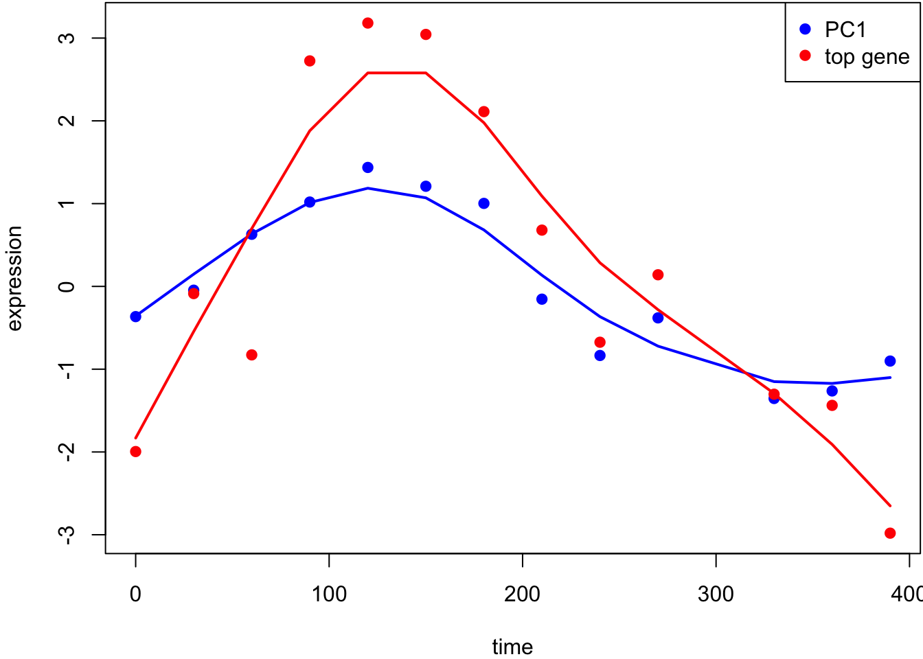
> dat <- t(scale(t(gene_expression), center=TRUE, scale=FALSE))Test for associations between PC1 and each gene, conditioning on PC1 and PC2 being relevant sources of systematic variation.
> jsobj <- jackstraw_pca(dat, r1=1, r=2, B=500, s=50, verbose=FALSE)
> jsobj$p.value %>% qvalue() %>% hist()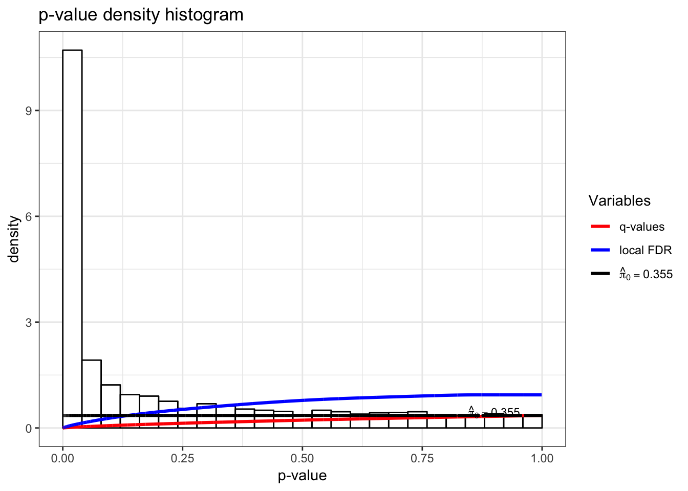
This is the most significant gene plotted with PC1.
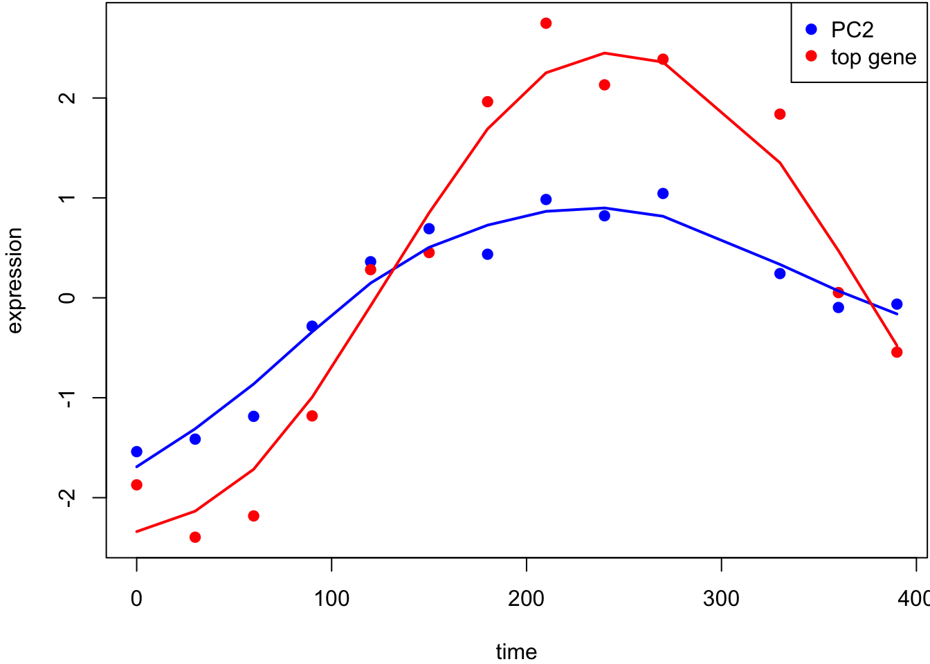
Test for associations between PC2 and each gene, conditioning on PC1 and PC2 being relevant sources of systematic variation.
> jsobj <- jackstraw_pca(dat, r1=2, r=2, B=500, s=50, verbose=FALSE)
> jsobj$p.value %>% qvalue() %>% hist()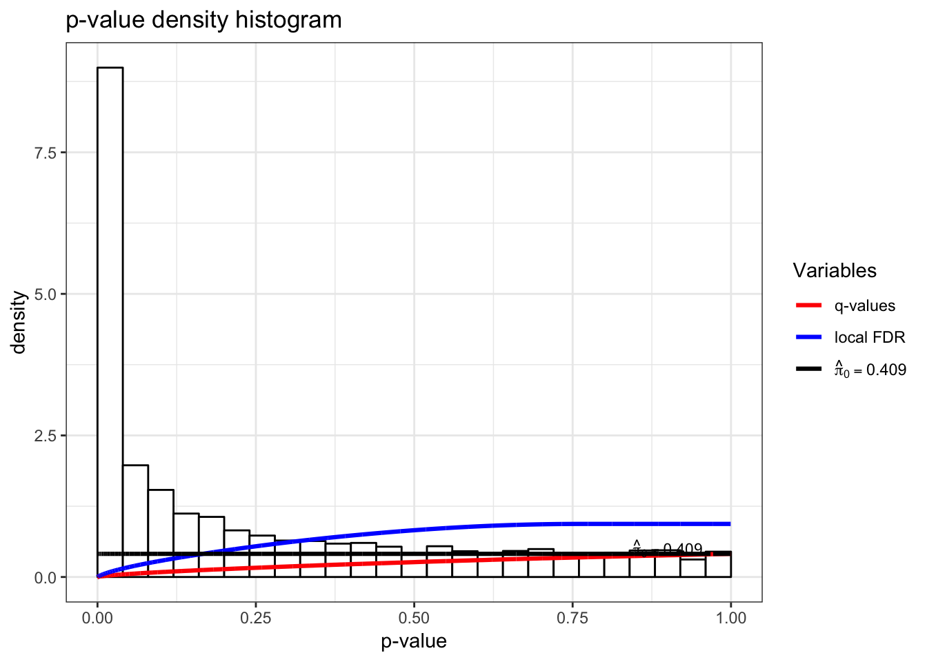
This is the most significant gene plotted with PC2.