QCB 508 – Week 3
John D. Storey
Spring 2017

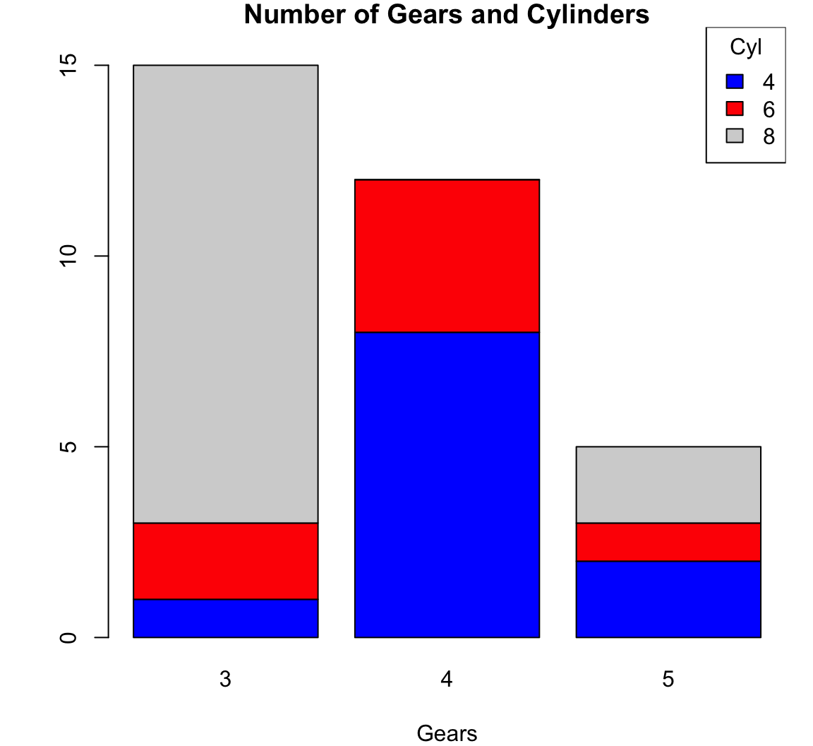
Barplot
> cyl_tbl <- table(mtcars$cyl)
> barplot(cyl_tbl, xlab="Cylinders", ylab="Count")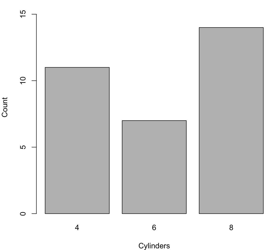
Boxplot
> boxplot(mtcars$mpg, ylab="MPG", col="lightgray")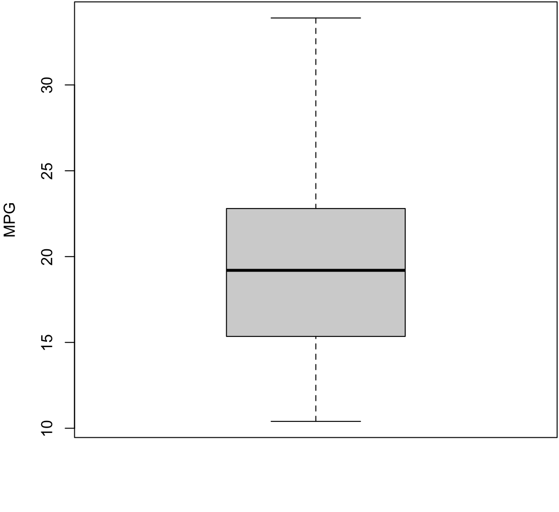
Boxplot with Outliers
> boxplot(mtcars$wt, ylab="Weight (1000 lbs)",
+         col="lightgray")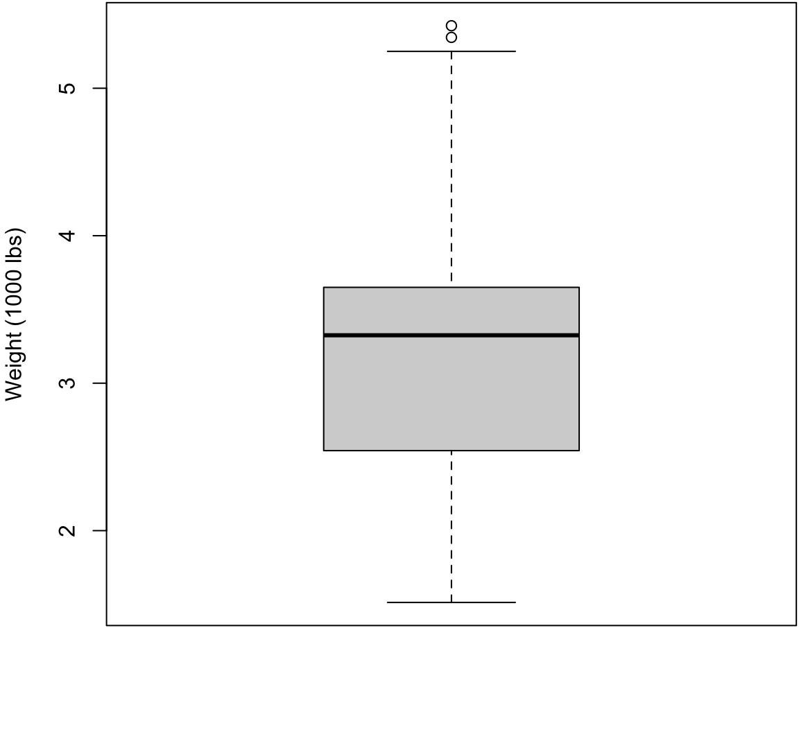
Histogram
> hist(mtcars$mpg, xlab="MPG", main="", col="lightgray")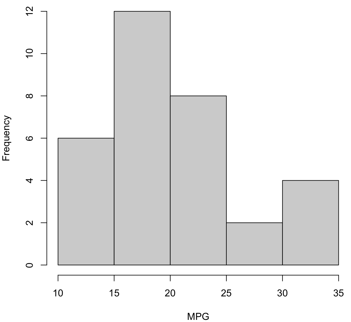
Histogram with More Breaks
> hist(mtcars$mpg, breaks=12, xlab="MPG", main="", col="lightgray")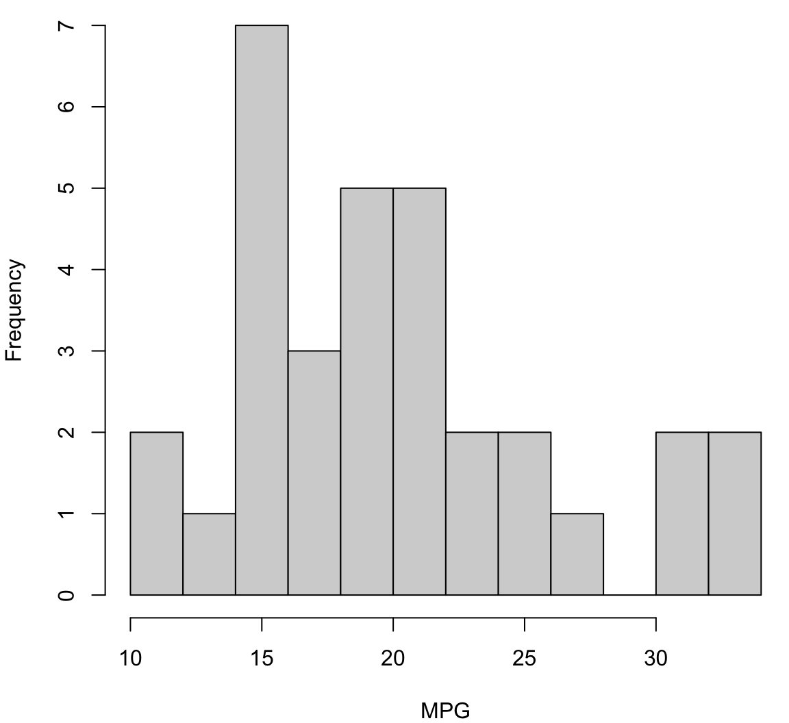
Density Plot
> plot(density(mtcars$mpg), xlab="MPG", main="")
> polygon(density(mtcars$mpg), col="lightgray", border="black")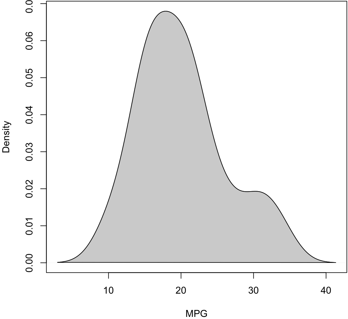
Boxplot (Side-By-Side)
> boxplot(mpg ~ cyl, data=mtcars, xlab="Cylinders",
+         ylab="MPG", col="lightgray")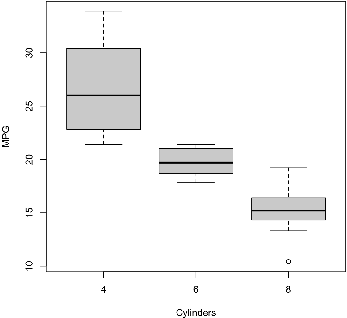
Scatterplot
> plot(mtcars$wt, mtcars$mpg, xlab="Weight (1000 lbs)",
+      ylab="MPG")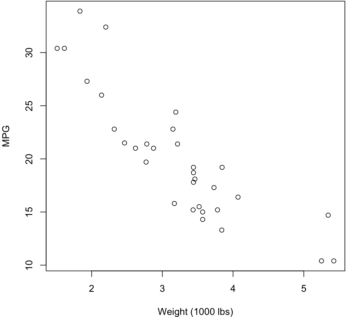
The geom_bar() layer forms a barplot and only requires an x assignment in the aes() call:
> ggplot(data = diamonds) +
+   geom_bar(mapping = aes(x = cut))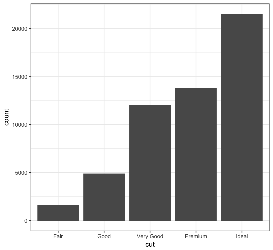
Color in the bars by assigning fill in geom_bar(), but outside of aes():
> ggplot(data = diamonds) +
+   geom_bar(mapping = aes(x = cut), fill = "tomato")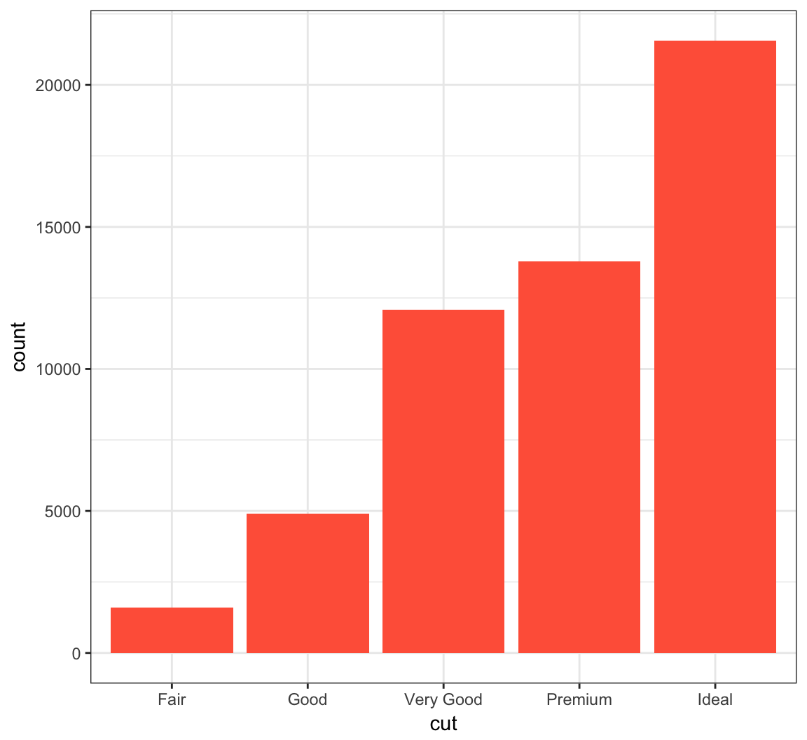
Color within the bars according to a variable by assigning fill in geom_bar() inside of aes():
> ggplot(data = diamonds) +
+   geom_bar(mapping = aes(x = cut, fill = cut))
When we use fill = clarity within aes(), we see that it shows the proportion of each clarity value within each cut value:
> ggplot(data = diamonds) +
+   geom_bar(mapping = aes(x = cut, fill = clarity))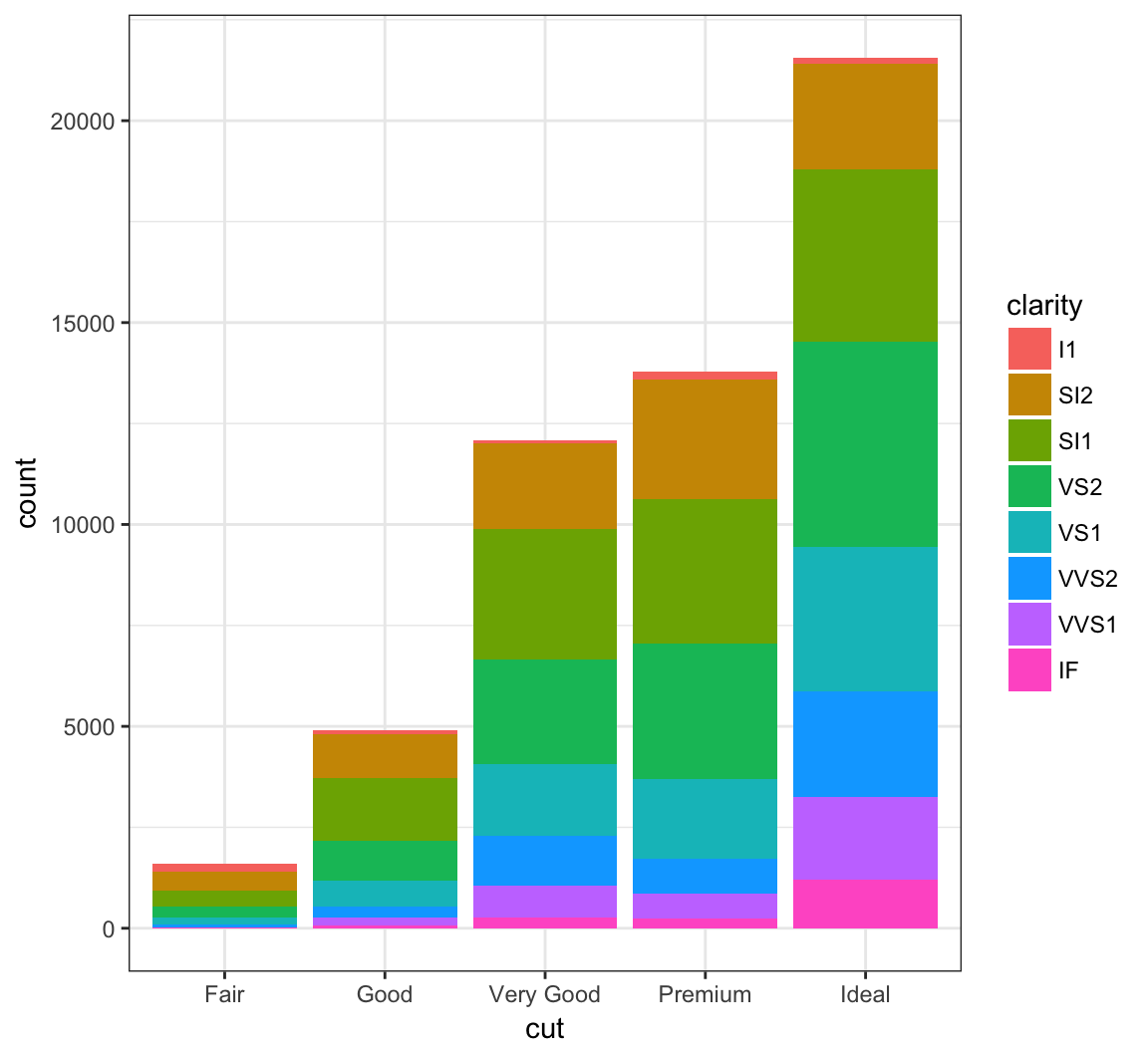
By setting position = "dodge" outside of aes(), it shows bar charts for the clarity values within each cut value:
> ggplot(data = diamonds) +
+   geom_bar(mapping= aes(x = cut, fill = clarity),
+            position = "dodge")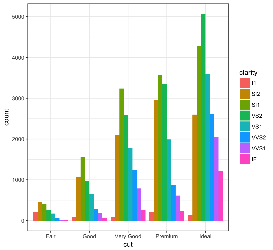
By setting position = "fill", it shows the proportion of clarity values within each cut value and no longer shows the cut values:
> ggplot(data = diamonds) +
+   geom_bar(mapping=aes(x = cut, fill = clarity),
+            position = "fill") +
+   labs(x = "cut", y = "relative proporition within cut")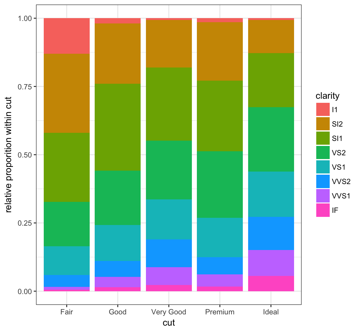
The geom_boxplot() layer forms a boxplot and requires both x and y assignments in the aes() call, even when plotting a single boxplot:
> ggplot(data = mpg) +
+   geom_boxplot(mapping = aes(x = 1, y = hwy))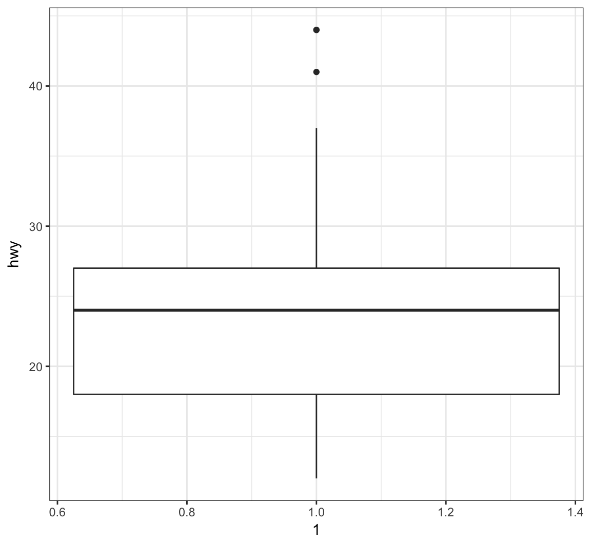
Color in the boxes by assigning fill in geom_boxplot(), but outside of aes():
> ggplot(data = mpg) +
+   geom_boxplot(mapping = aes(x = 1, y = hwy),
+                fill="lightblue") +
+   labs(x=NULL)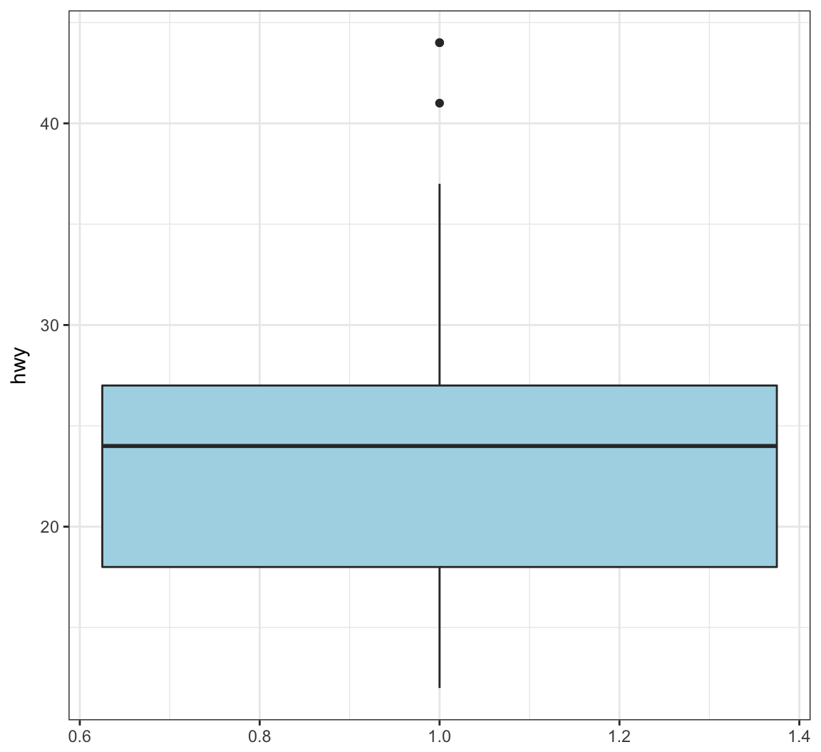
Show a boxplot for the y values occurring within each x factor level by making these assignments in aes():
> ggplot(data = mpg) +
+   geom_boxplot(mapping = aes(x = factor(cyl), y = hwy))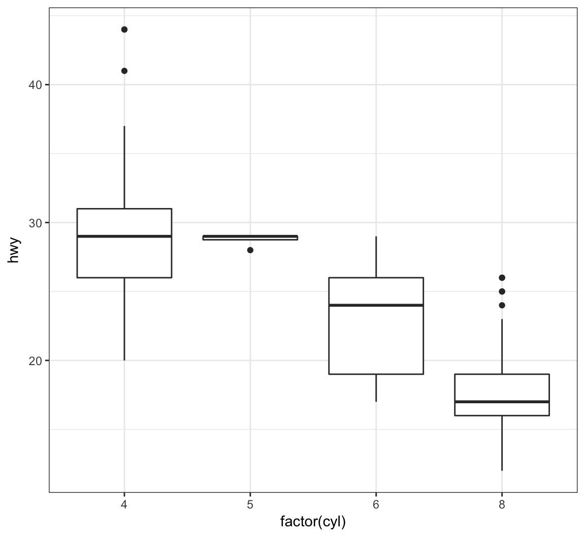
By assigning the fill argument within aes(), we can color each boxplot according to the x-axis factor variable:
> ggplot(data = mpg) +
+   geom_boxplot(mapping = aes(x = factor(cyl), y = hwy,
+                              fill = factor(cyl)))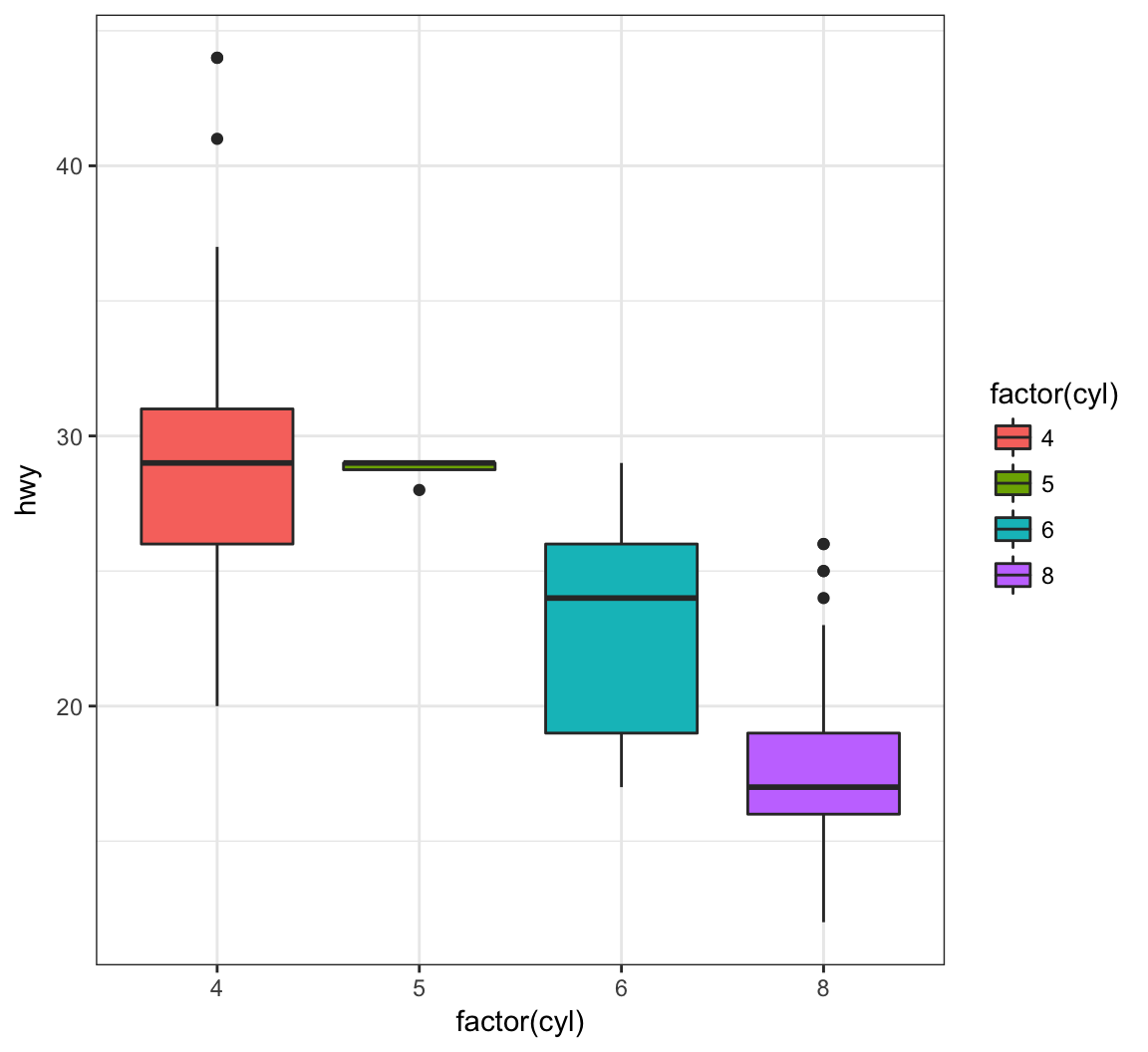
The geom_jitter() function plots the data points and randomly jitters them so we can better see all of the points:
> ggplot(data = mpg, mapping = aes(x=factor(cyl), y=hwy)) +
+   geom_boxplot(fill = "lightblue") +
+   geom_jitter(width = 0.2)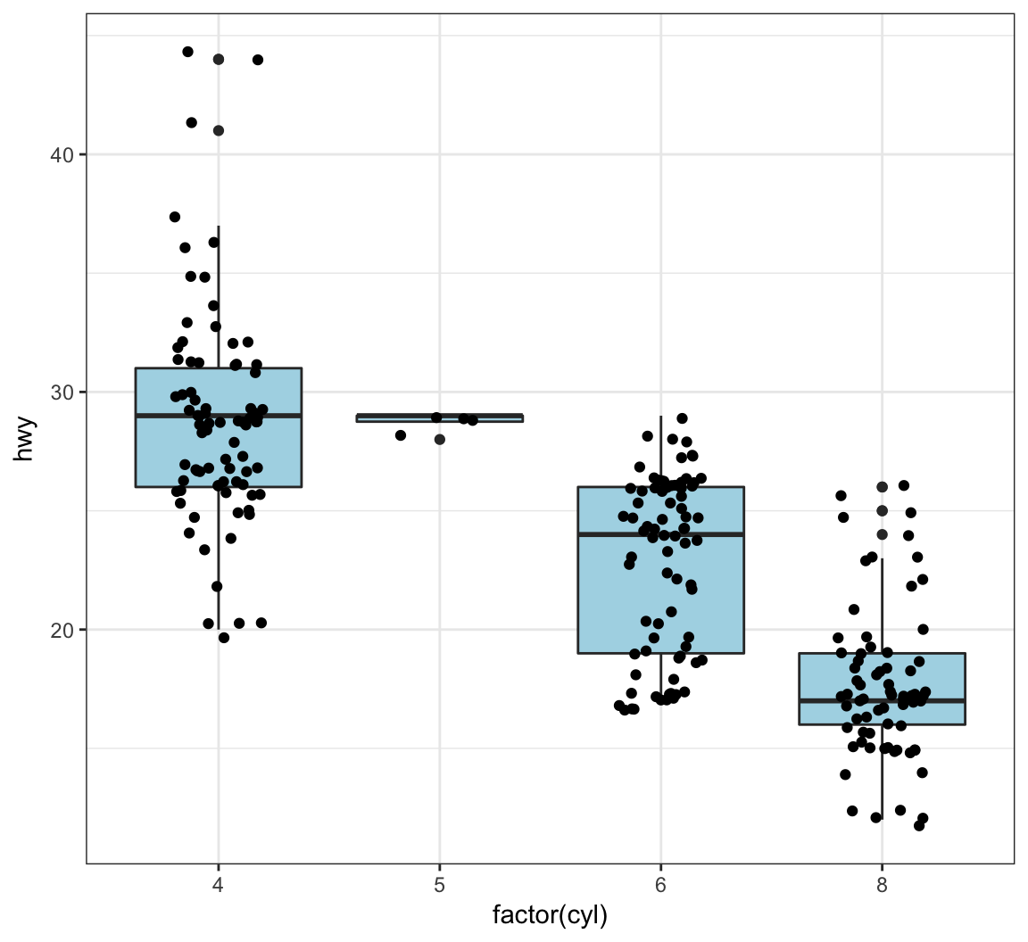
A violin plot, called via geom_violin(), is similar to a boxplot, except shows a density plot turned on its side and reflected across its vertical axis:
> ggplot(data = mpg) +
+   geom_violin(mapping = aes(x = drv, y = hwy))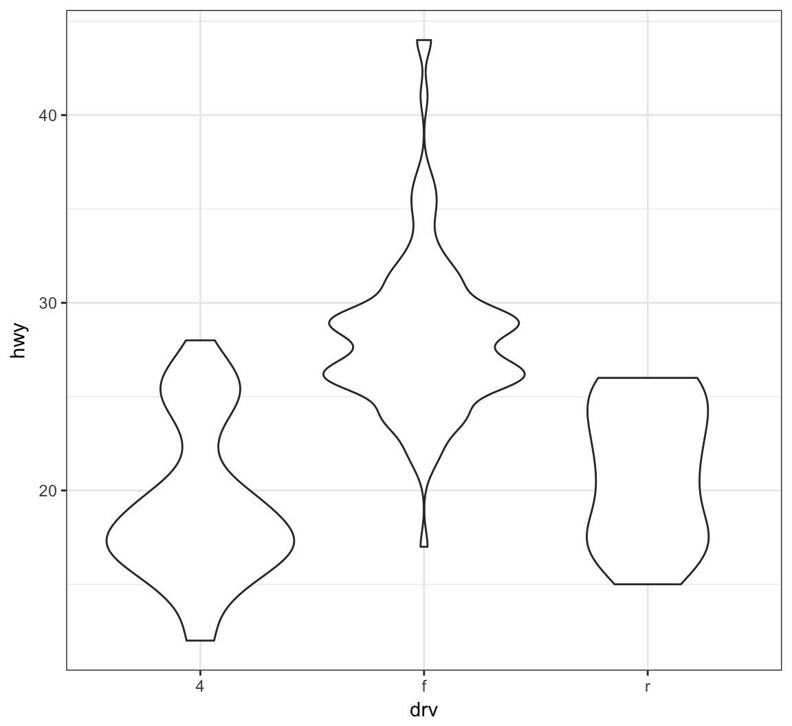
Add a geom_jitter() to see how the original data points relate to the violin plots:
> ggplot(data = mpg, mapping = aes(x = drv, y = hwy)) +
+   geom_violin(adjust=1.2) +
+   geom_jitter(width=0.2, alpha=0.5)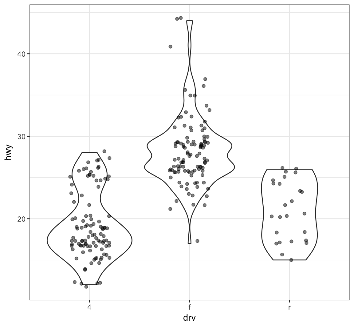
Boxplot example on the gapminder data:
> ggplot(gapminder, aes(x = continent, y = lifeExp)) +
+   geom_boxplot(outlier.colour = "red") +
+   geom_jitter(width = 0.1, alpha = 0.25)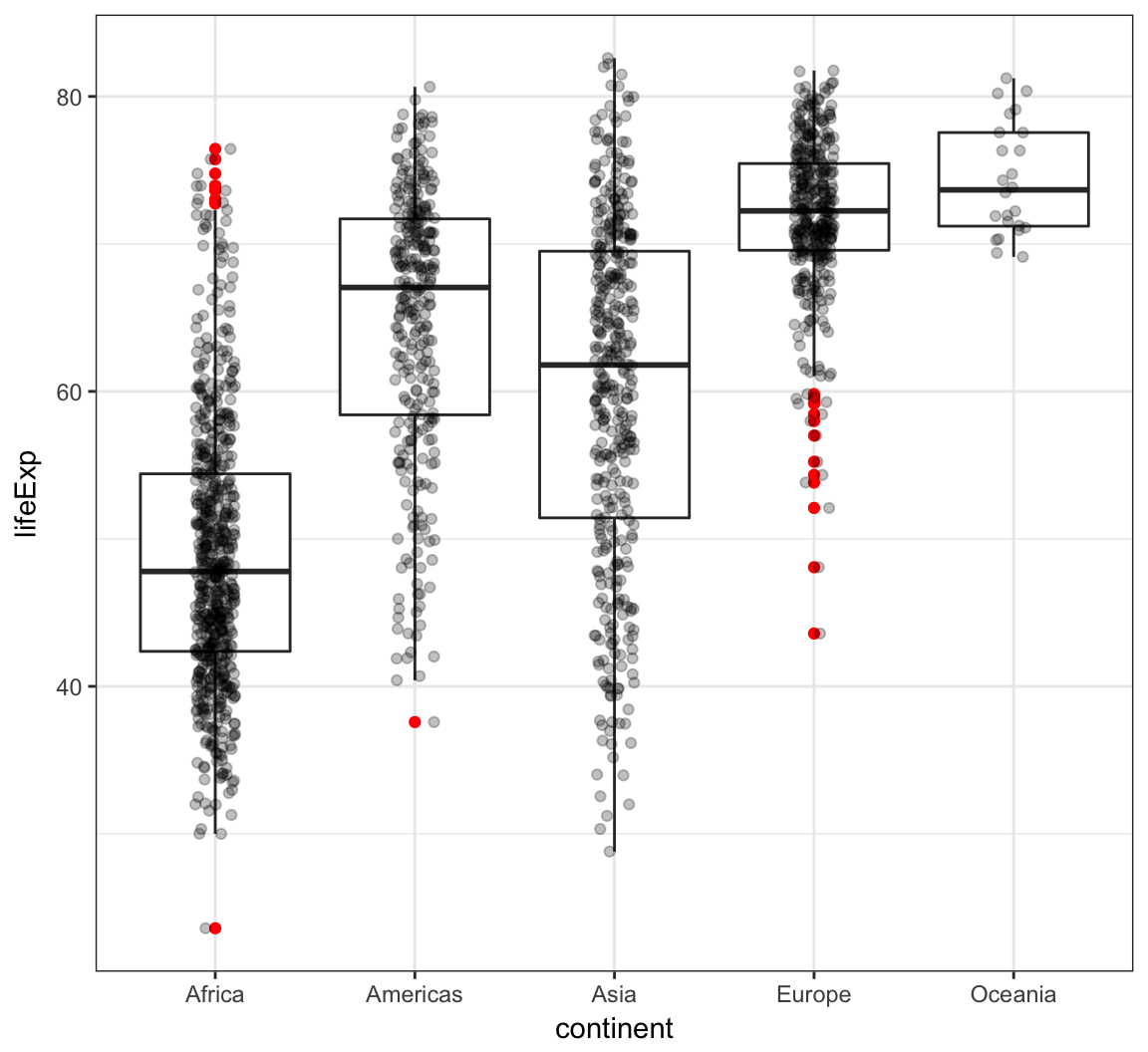
Analogous violin plot example on the gapminder data:
> ggplot(gapminder, aes(x = continent, y = lifeExp)) +
+   geom_violin() +
+   geom_jitter(width = 0.1, alpha = 0.25)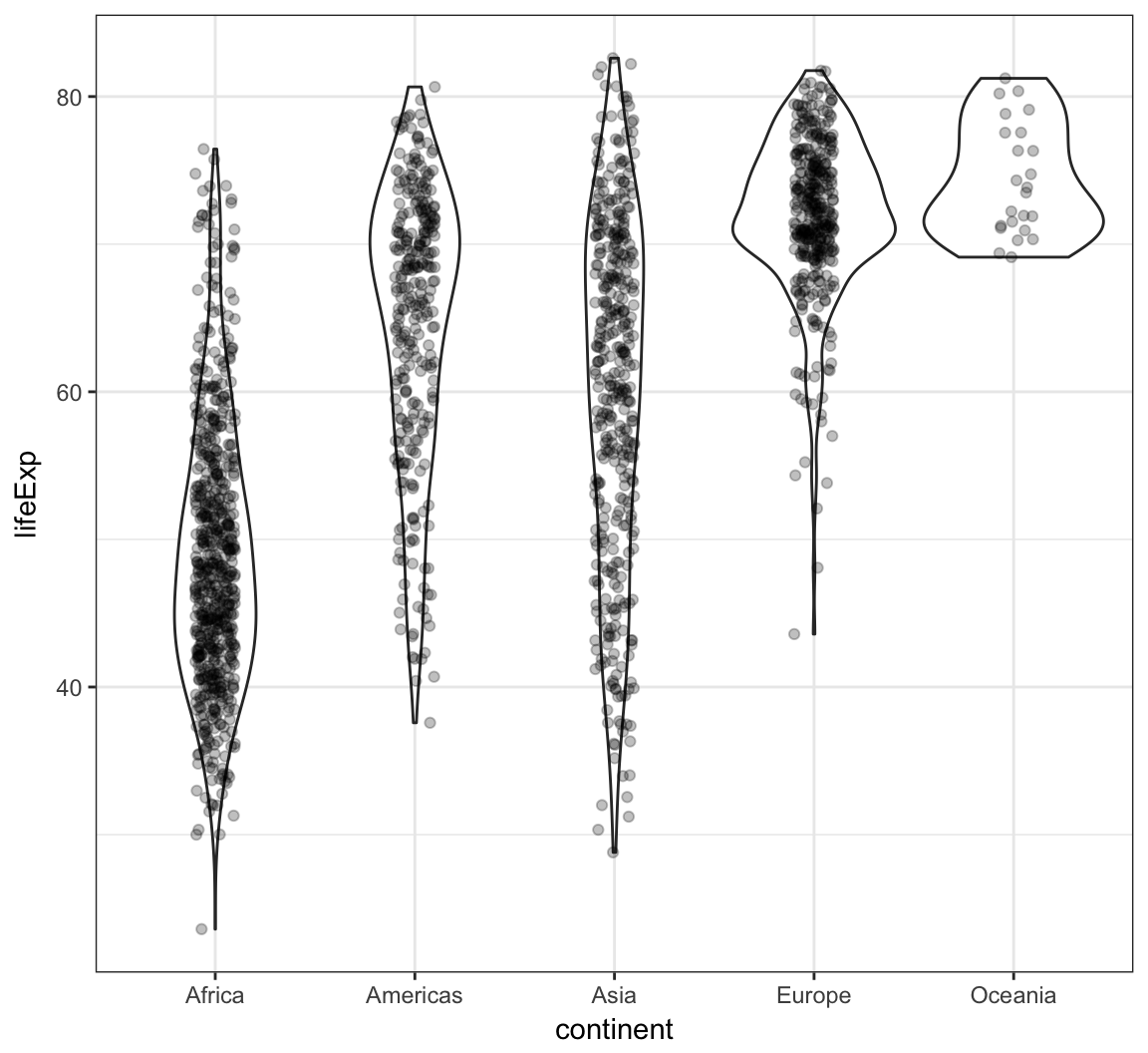
We can create a histogram using the geom_histogram() layer, which requires an x argument only in the aes() call:
> ggplot(gapminder) +
+   geom_histogram(mapping = aes(x=lifeExp))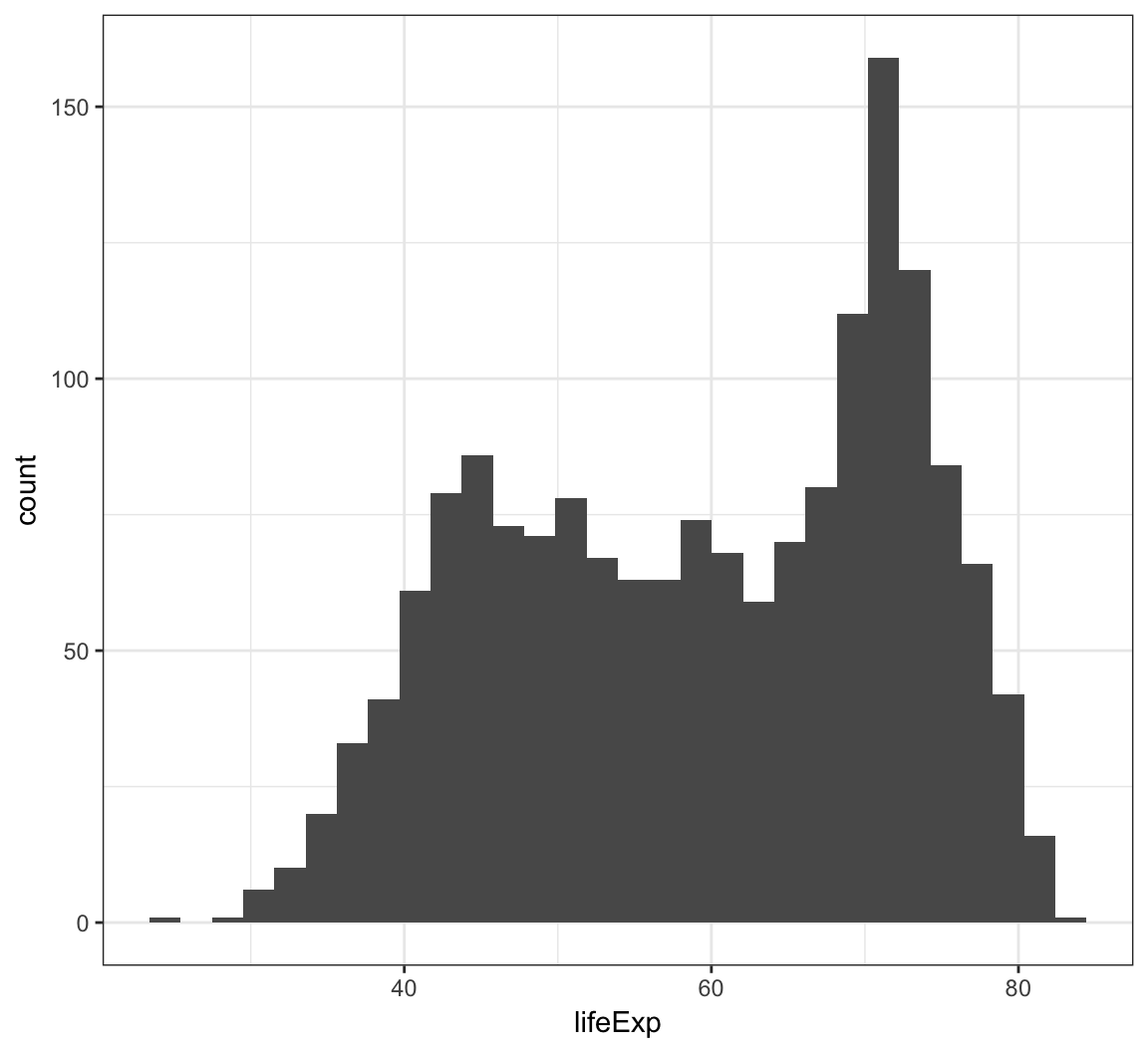
We can change the bin width directly in the histogram, which is an intuitive parameter to change based on visual inspection:
> ggplot(gapminder) +
+   geom_histogram(mapping = aes(x=lifeExp), binwidth=5)
The bins are sometimes centered in an unexpected manner in ggplot2:
> ggplot(diamonds) +
+   geom_histogram(mapping = aes(x=price), binwidth = 1000)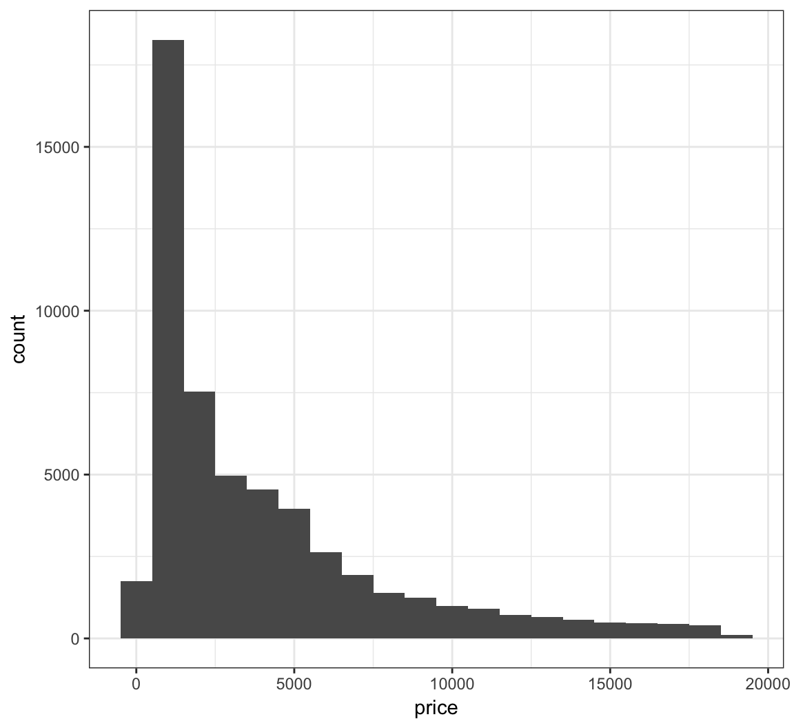
Let’s fix how the bins are centered (make center half of binwidth).
> ggplot(diamonds) +
+   geom_histogram(mapping = aes(x=price), binwidth = 1000,
+                  center=500)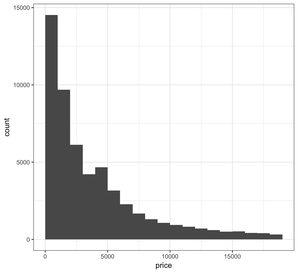
Instead of counts on the y-axis, we may instead want the area of the bars to sum to 1, like a probability density:
> ggplot(gapminder) +
+   geom_histogram(mapping = aes(x=lifeExp, y=..density..),
+                  binwidth=5)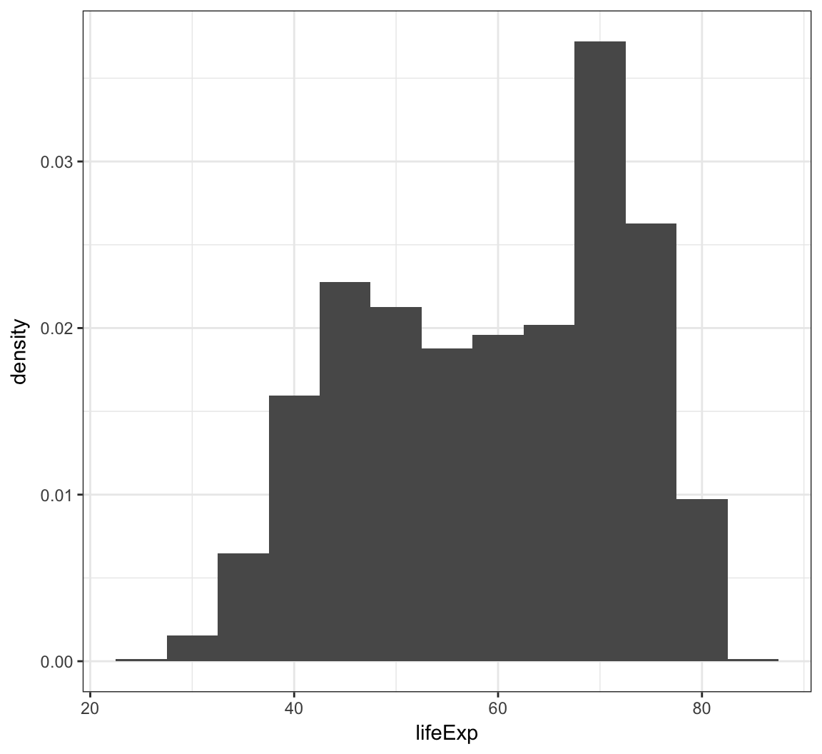
When we use fill = continent within aes(), we see that it shows the counts of each continent value within each lifeExp bin:
> ggplot(gapminder) +
+   geom_histogram(mapping = aes(x=lifeExp, fill = continent),
+                  binwidth = 5)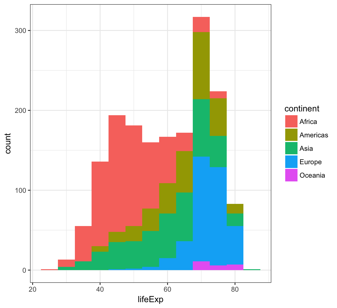
Display a density plot using the geom_density() layer:
> ggplot(gapminder) +
+   geom_density(mapping = aes(x=lifeExp))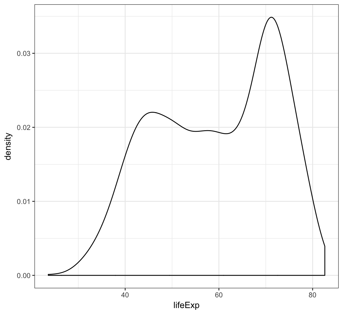
Employ the arguments color="blue" and fill="lightblue" outside of the aes() call to include some colors:
> ggplot(gapminder) +
+   geom_density(mapping = aes(x=lifeExp), color="blue",
+                fill="lightblue")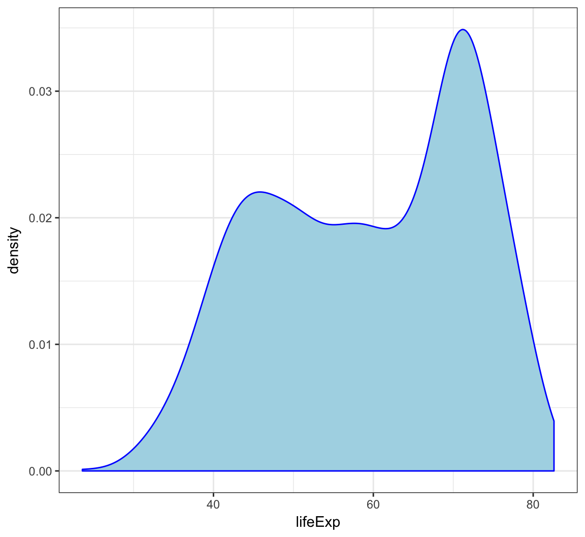
By utilizing color=as.factor(year) we plot a density of lifeExp stratified by each year value:
> ggplot(gapminder) +
+   geom_density(aes(x=lifeExp, color=as.factor(year)),
+                size=1.2)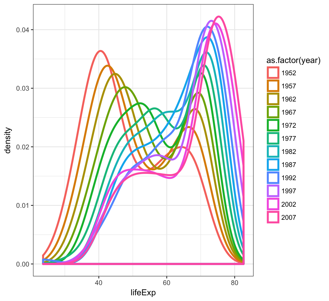
Overlay a density plot and a histogram together:
> ggplot(gapminder, mapping = aes(x=lifeExp)) +
+   geom_histogram(aes(y=..density..), color="black",
+                  fill="white") +
+   geom_density(fill="lightblue", alpha=.5)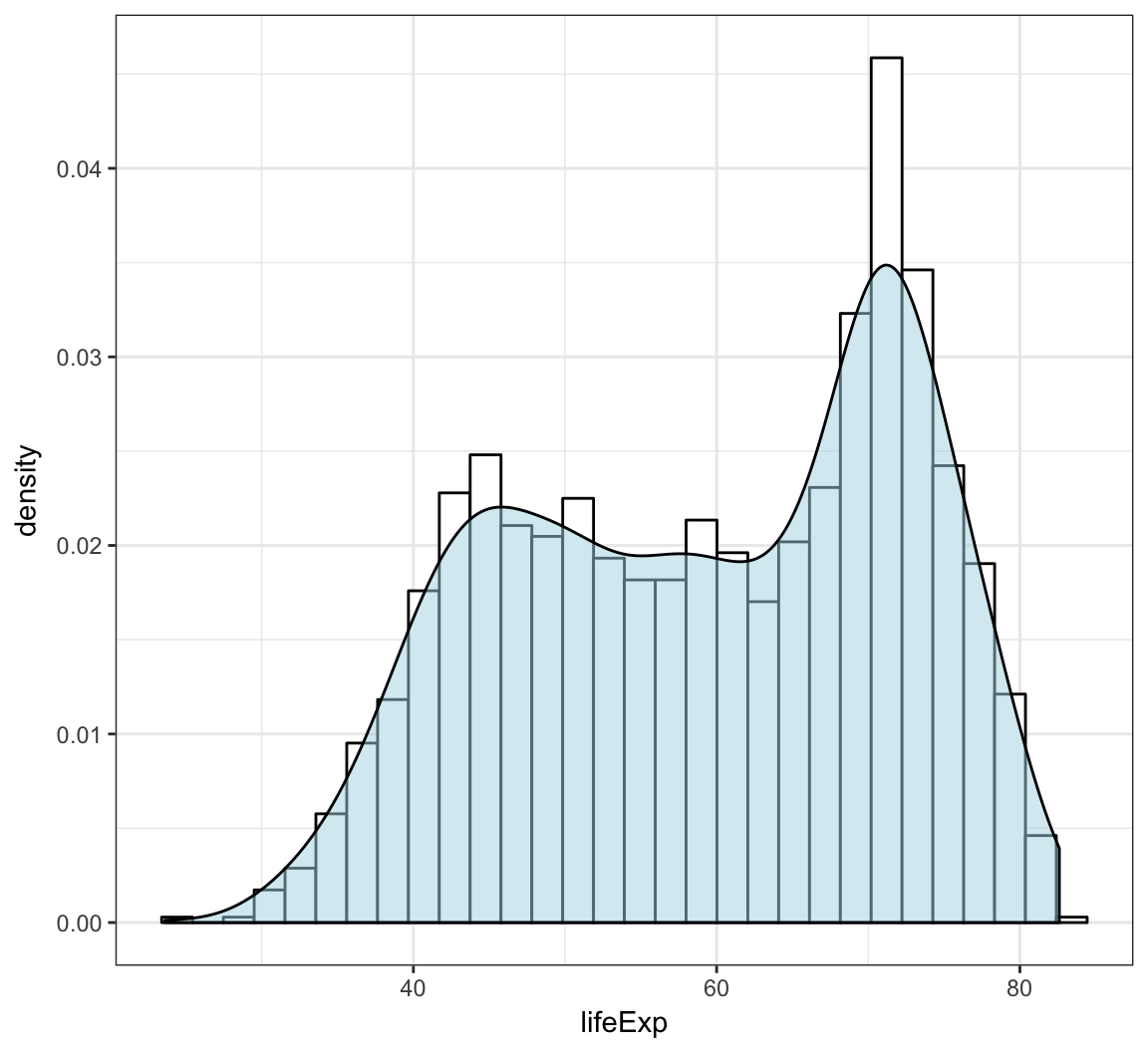
We can geom_lines() to plot a line showing the popularity of “John” over time:
> ggplot(data = john) +
+   geom_line(mapping = aes(x=year, y=prop), size=1.5)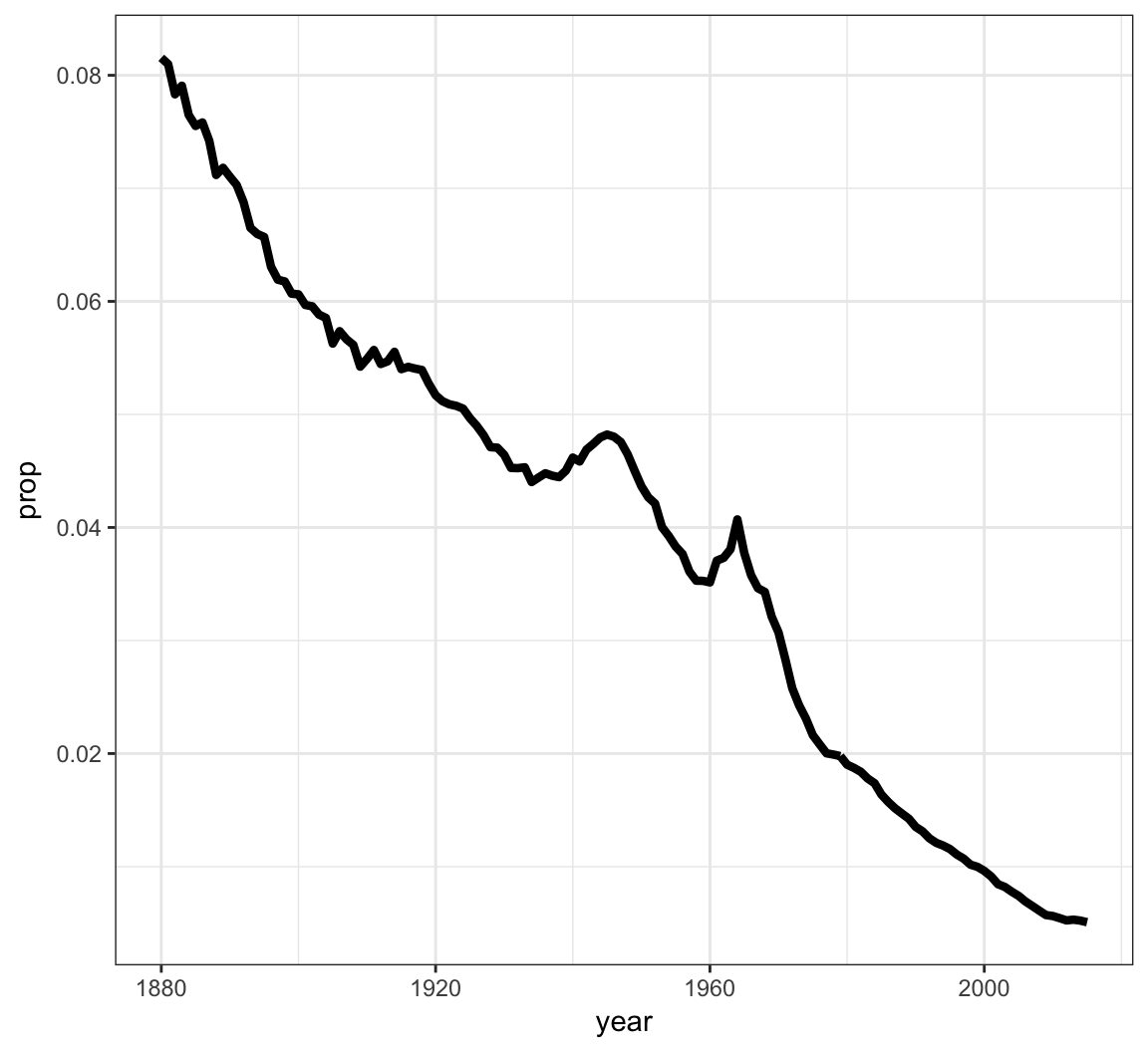
Now let’s look at a name that occurs nontrivially in males and females:
> kelly <- babynames %>% filter(name=="Kelly")
> ggplot(data = kelly) +
+   geom_line(mapping = aes(x=year, y=prop, color=sex),
+             size=1.5)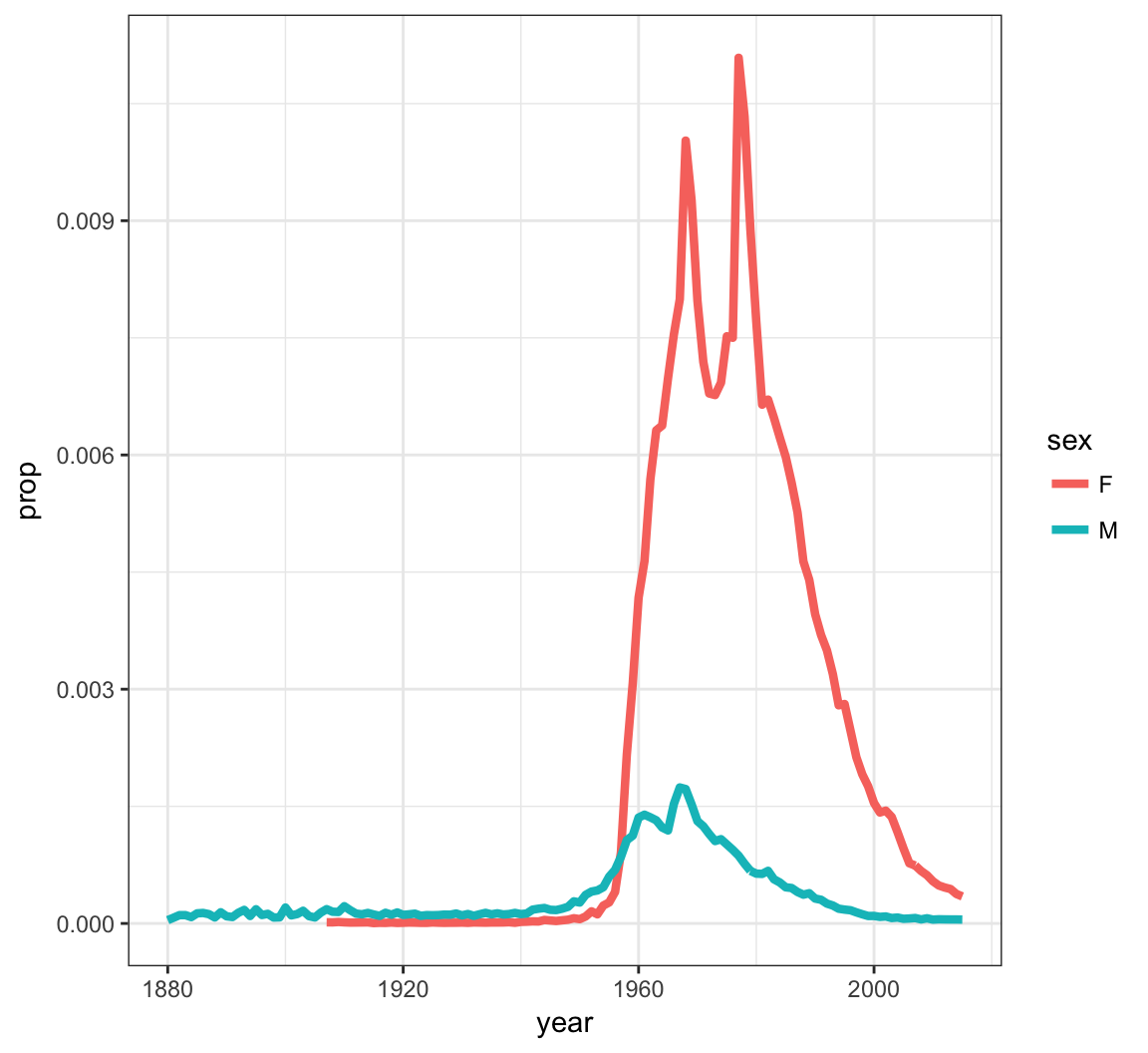
The layer geom_point() produces a scatterplot, and the aes() call requires x and y assignment:
> ggplot(data = mpg) +
+   geom_point(mapping = aes(x = displ, y = hwy))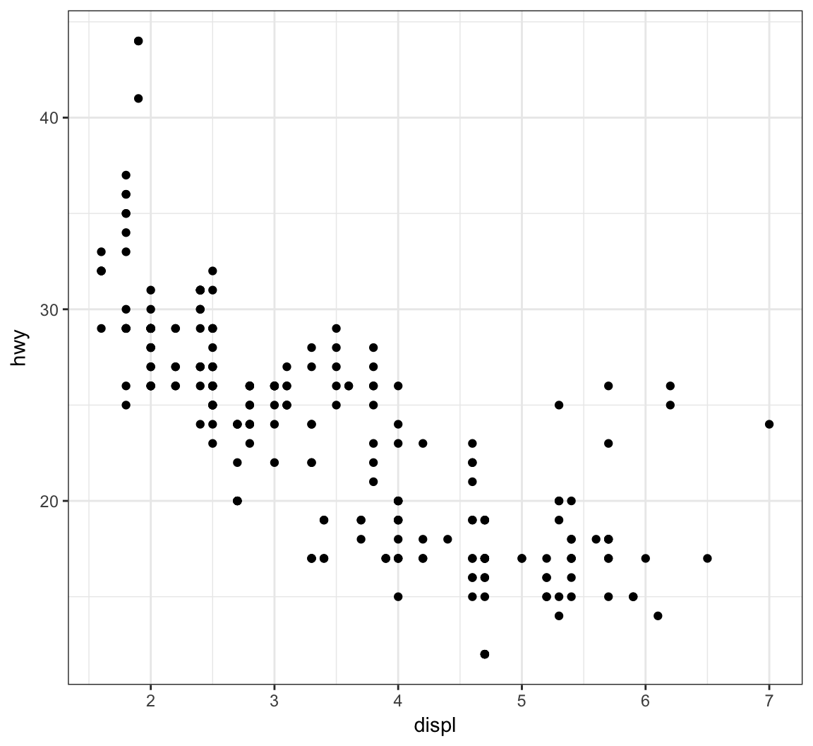
Give the points a color:
> ggplot(data = mpg) +
+   geom_point(mapping = aes(x = displ, y = hwy),
+              color = "blue")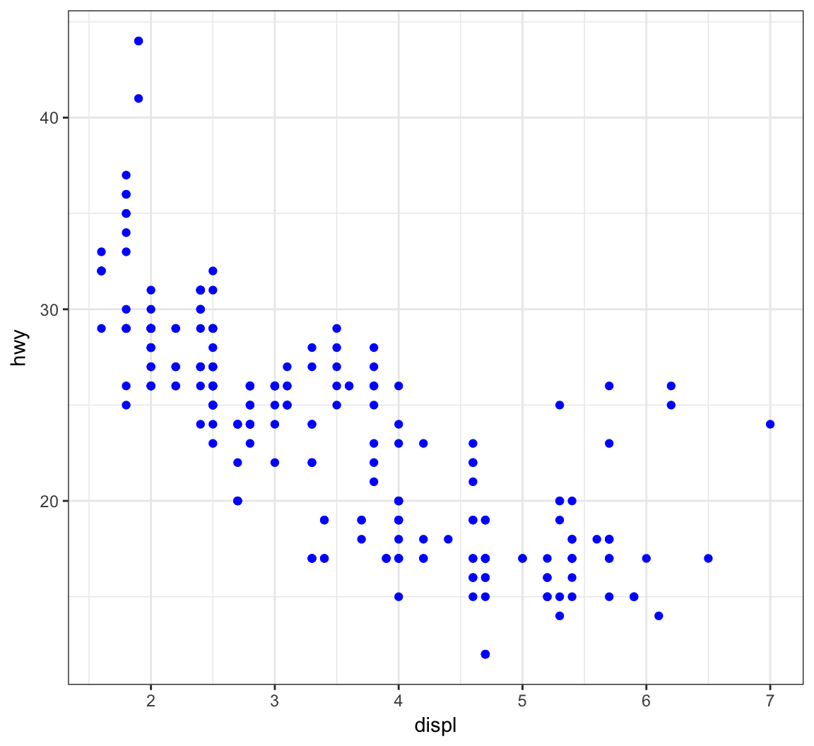
Color the points according to a factor variable by including color = class within the aes() call:
> ggplot(data = mpg) +
+   geom_point(mapping = aes(x = displ, y = hwy,
+                            color = class))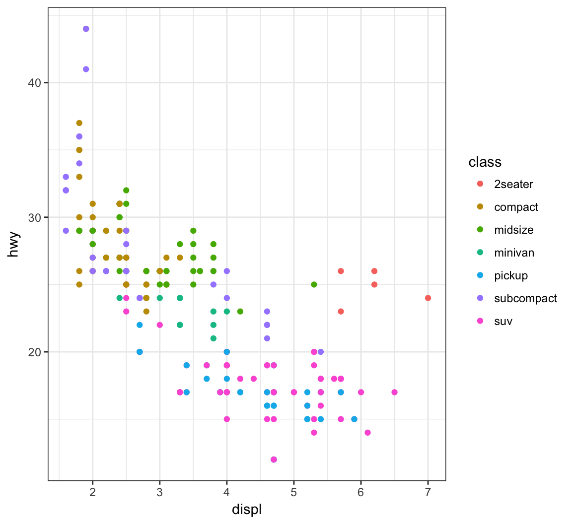
Increase the size of points with size=2 outside of the aes() call:
> ggplot(data = mpg) +
+   geom_point(mapping = aes(x = displ, y = hwy,
+                            color = class), size=2)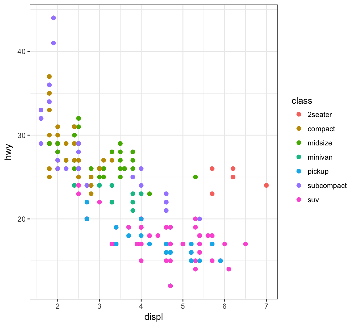
Vary the size of the points according to the pop variable:
> gapminder %>% filter(year==2007) %>% ggplot() +
+   geom_point(aes(x = log(gdpPercap), y = lifeExp,
+                  size = pop))
Vary the transparency of the points according to the class factor variable by setting alpha=class within the aes() call:
> ggplot(data = mpg) +
+   geom_point(mapping = aes(x = displ, y = hwy,
+                            alpha = class))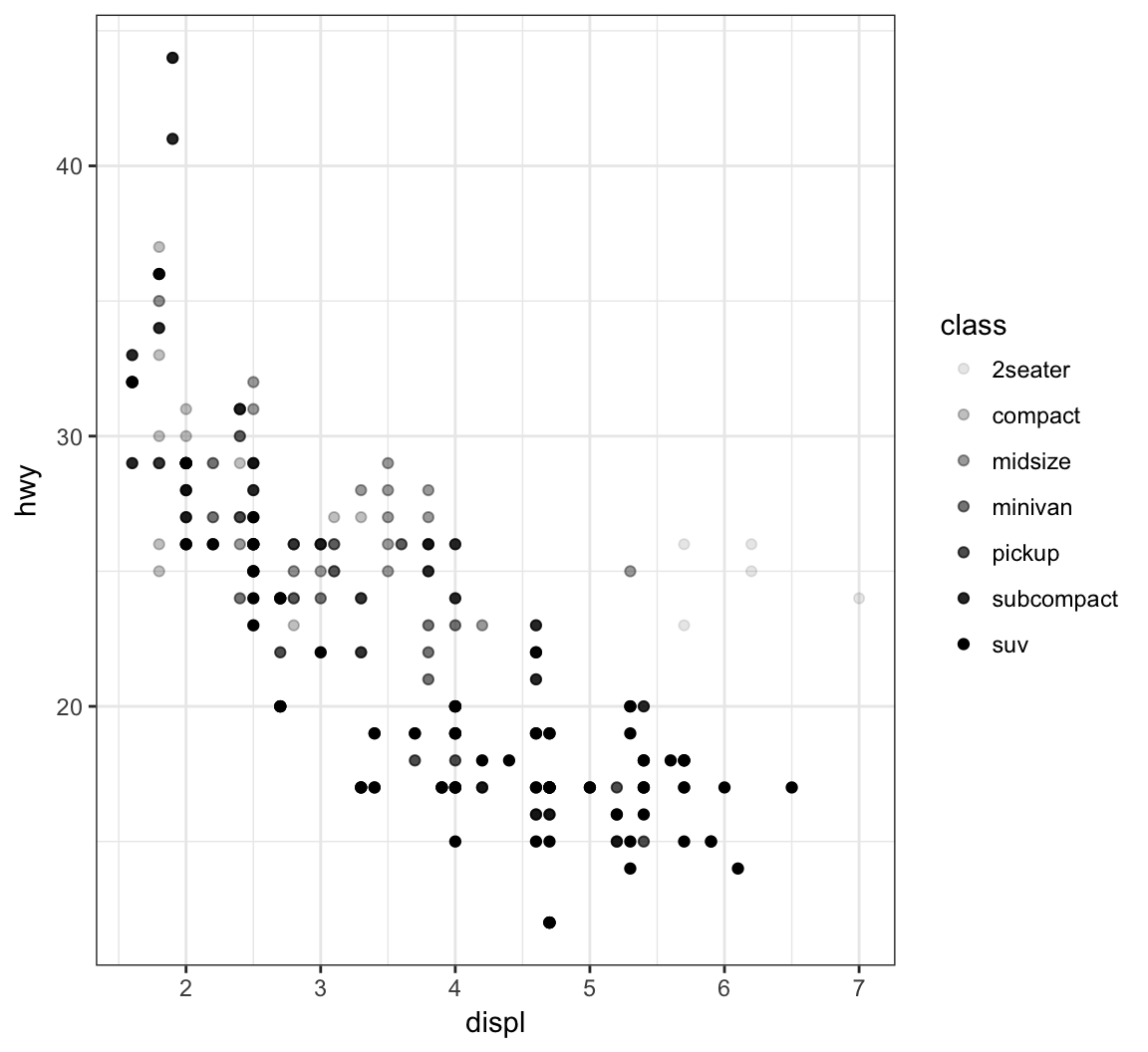
Vary the shape of the points according to the class factor variable by setting alpha=class within the aes() call (maximum 6 possible shapes – oops!):
> ggplot(data = mpg) +
+   geom_point(mapping = aes(x = displ, y = hwy,
+                            shape = class))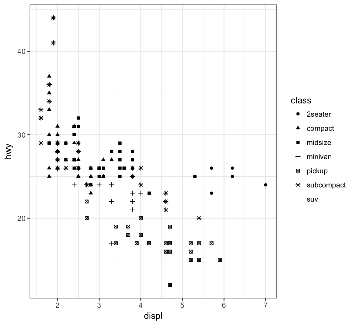
Color the points according to the cut variable by setting color=cut within the aes() call:
> ggplot(data = diamonds) +
+   geom_point(mapping = aes(x=carat, y=price, color=cut),
+              alpha=0.7)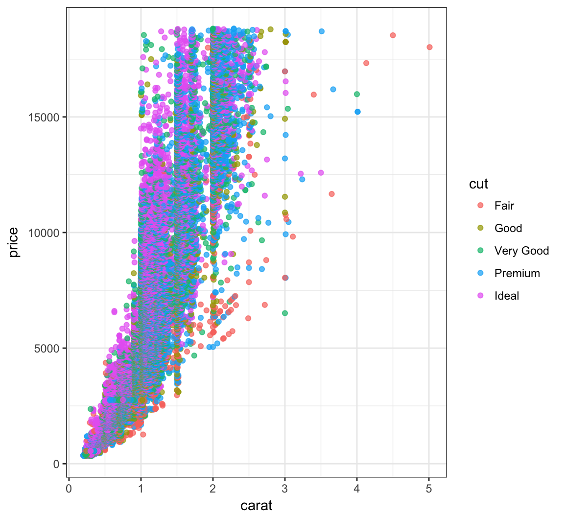
Color the points according to the clarity variable by setting color=clarity within the aes() call:
> ggplot(data = diamonds) +
+   geom_point(mapping=aes(x=carat, y=price, color=clarity),
+              alpha=0.3)
Override the alpha=0.3 in the legend:
> ggplot(data=diamonds) +
+   geom_point(mapping=aes(x=carat, y=price, color=clarity),
+              alpha=0.3) +
+   guides(color=guide_legend(override.aes = list(alpha = 1)))
A different way to take the log of gdpPercap:
> gapminder %>% filter(year==2007) %>% ggplot() +
+   geom_point(aes(x = gdpPercap, y = lifeExp,
+                  size = pop)) +
+   scale_x_log10()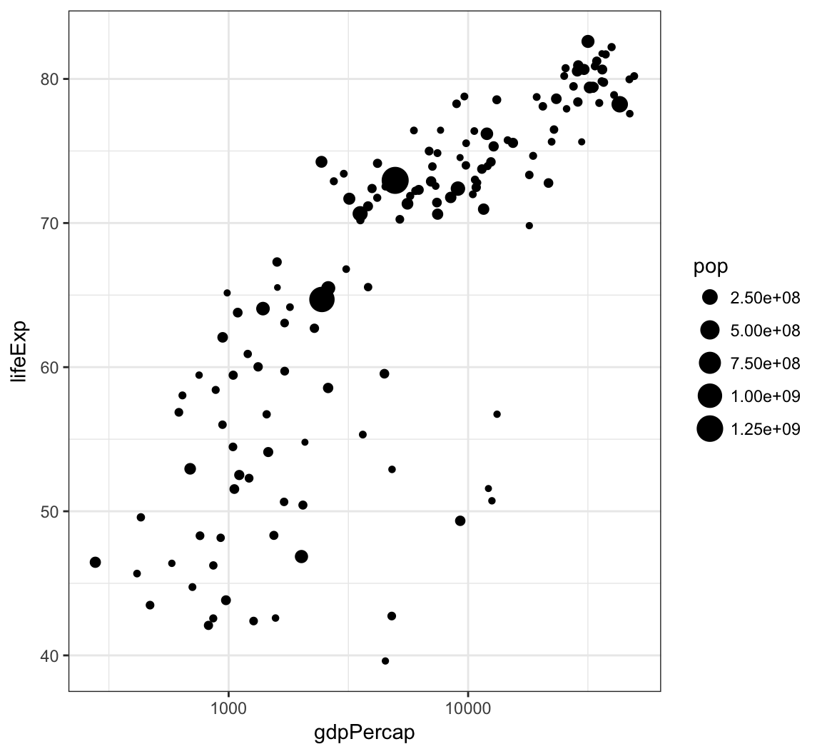
The price variable seems to be significantly right-skewed:
> ggplot(diamonds) +
+ geom_boxplot(aes(x=color, y=price)) 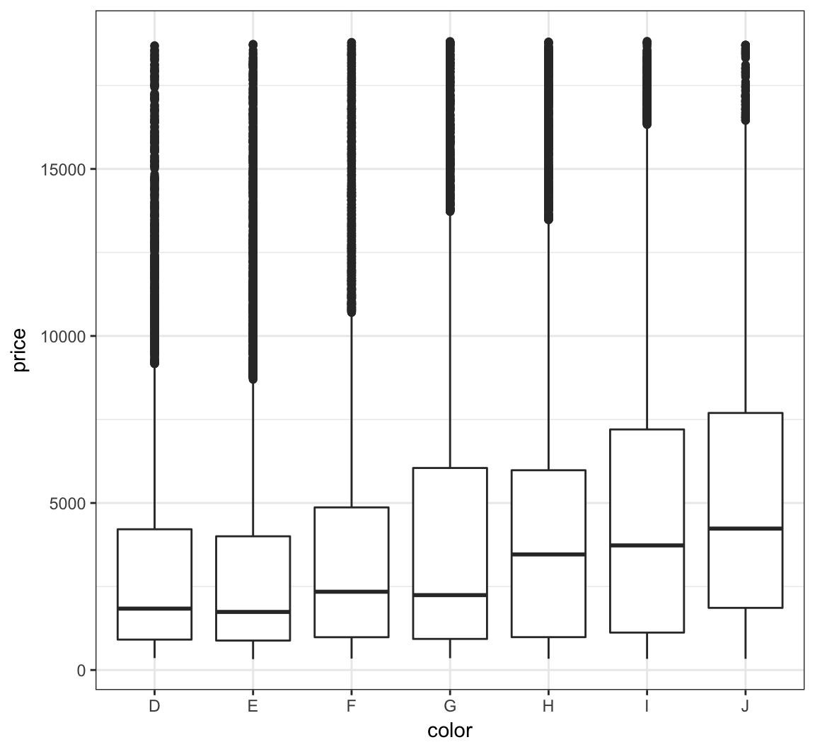
We can try to reduce this skewness by rescaling the variables. We first try to take the log(base=10) of the price variable via scale_y_log10():
> ggplot(diamonds) +
+   geom_boxplot(aes(x=color, y=price)) +
+   scale_y_log10()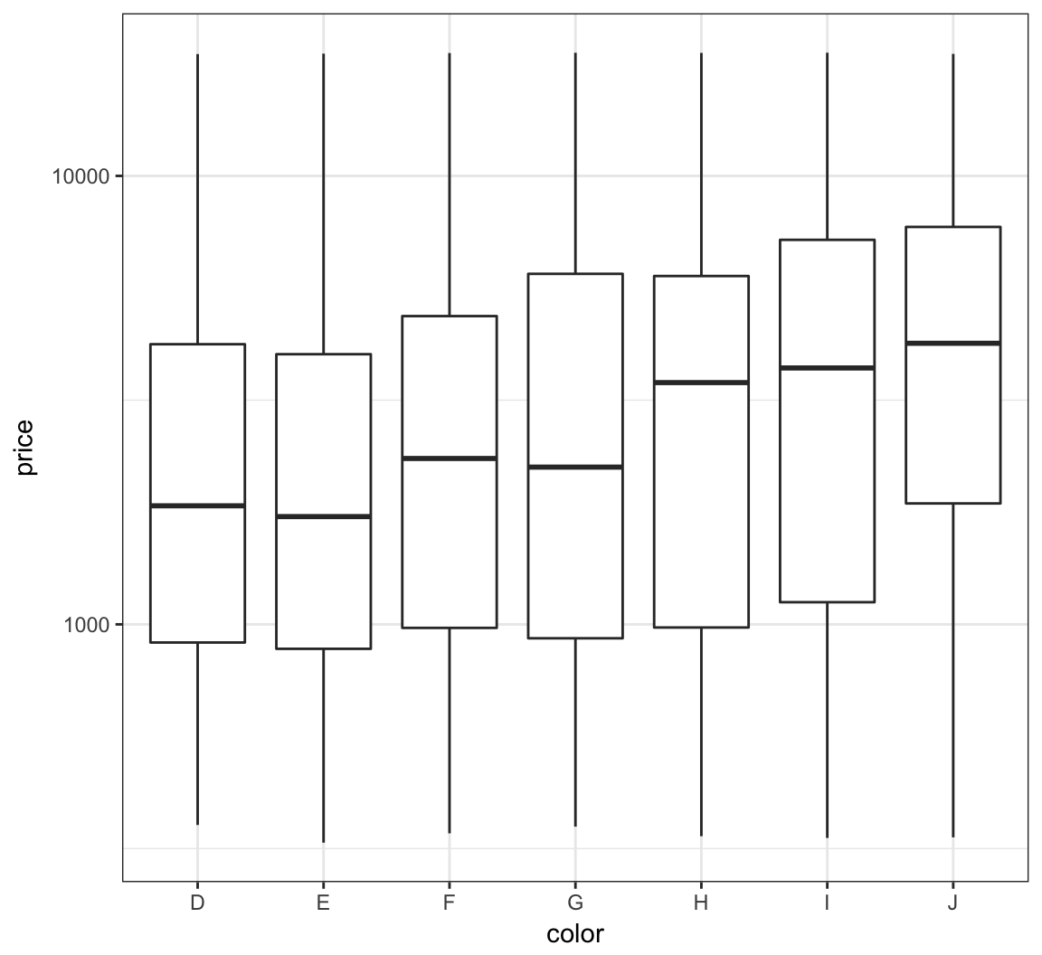
Let’s repeat this on the analogous violing plots:
> ggplot(diamonds) +
+   geom_violin(aes(x=color, y=price)) +
+   scale_y_log10()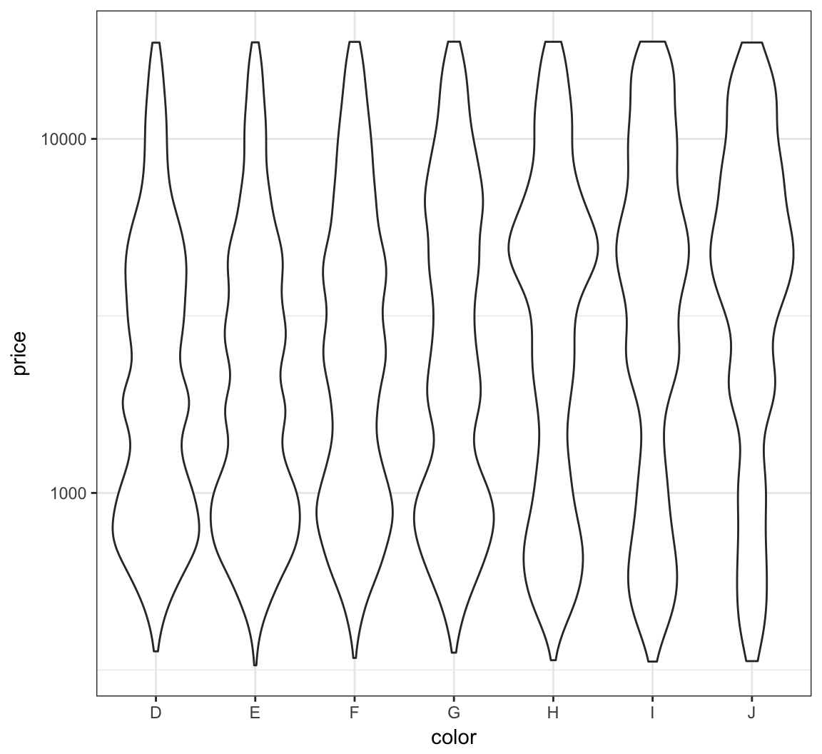
The relationship between carat and price is nonlinear. Let’s explore different transformations to find an approximately linear relationship.
> ggplot(data = diamonds) +
+   geom_point(mapping=aes(x=carat, y=price, color=clarity),
+              alpha=0.3)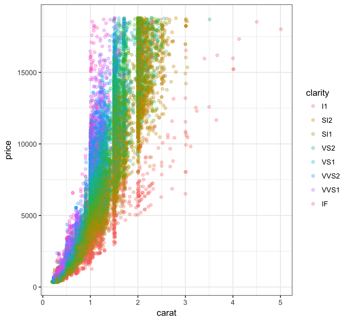
First try to take the squareroot of the the price variable:
> ggplot(data = diamonds) +
+   geom_point(aes(x=carat, y=price, color=clarity),
+              alpha=0.3) +
+   scale_y_sqrt()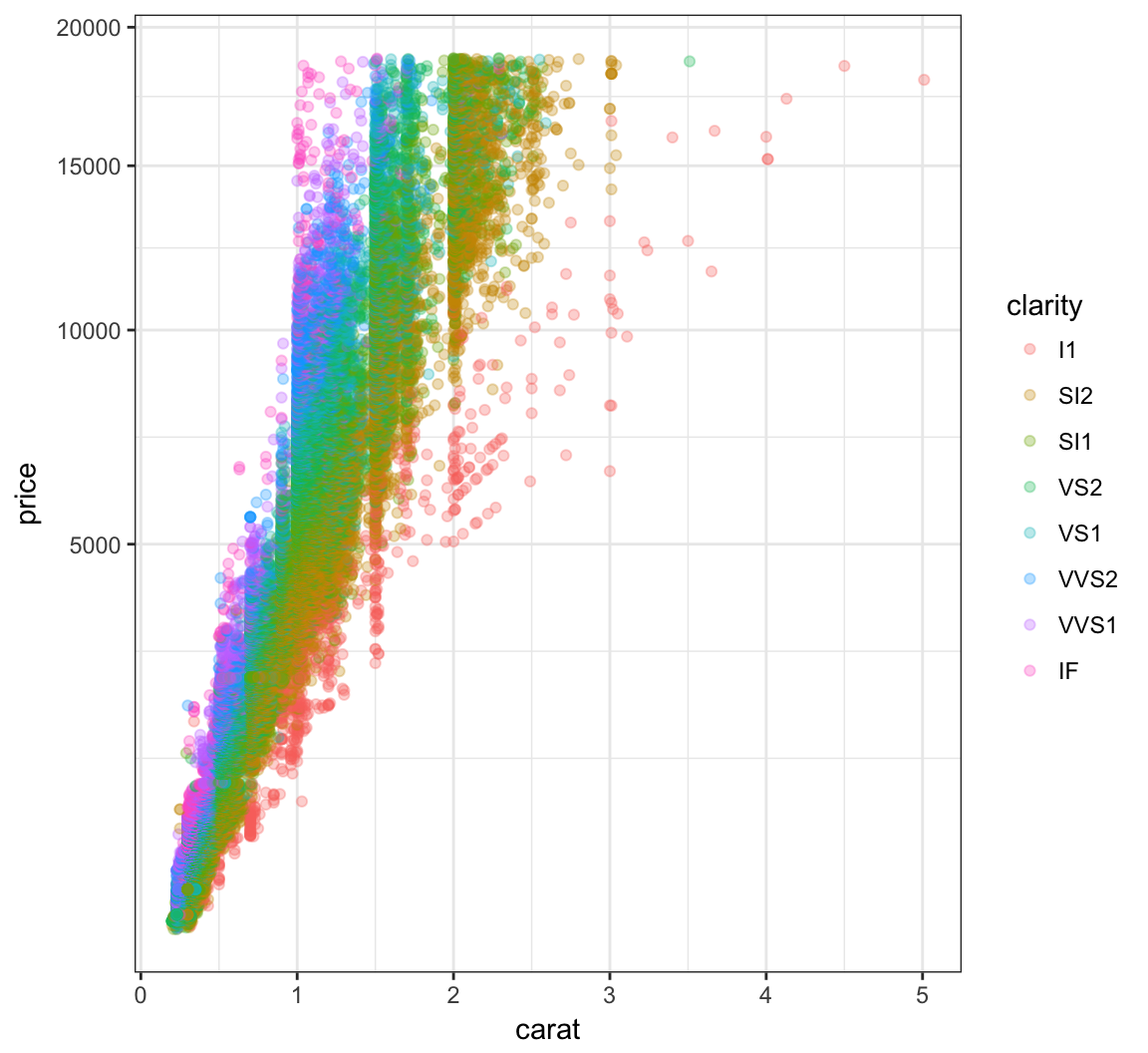
Now let’s try to take log(base=10) on both the carat and price variables:
> ggplot(data = diamonds) +
+   geom_point(aes(x=carat, y=price, color=clarity), alpha=0.3) +
+   scale_y_log10(breaks=c(1000,5000,10000)) +
+   scale_x_log10(breaks=1:5)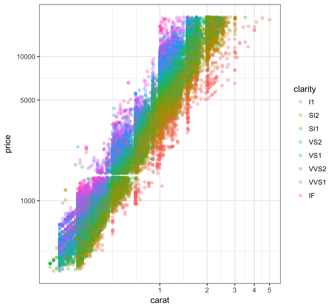
Forming a violin plot of price stratified by clarity and transforming the price variable yields an interesting relationship in this data set:
> ggplot(diamonds) +
+   geom_violin(aes(x=clarity, y=price, fill=clarity),
+               adjust=1.5) +
+   scale_y_log10()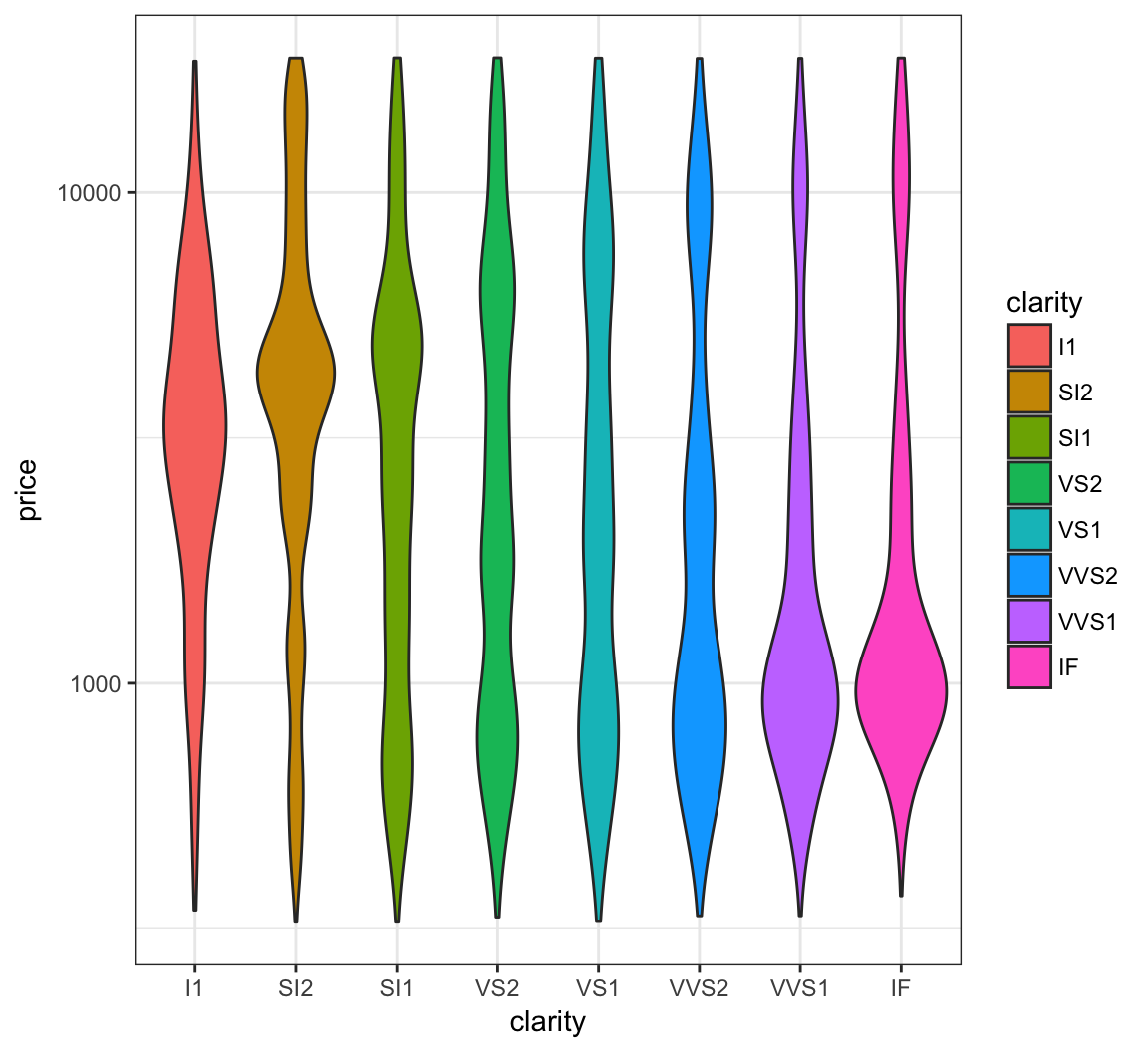
Recall the scatterplot showing the relationship between highway mpg and displacement. How can we plot a smoothed relationship between these two variables?
> ggplot(data = mpg) +
+   geom_point(mapping = aes(x = displ, y = hwy))
Plot a smoother with geom_smooth() using the default settings (other than removing the error bands):
> ggplot(data = mpg, mapping = aes(x = displ, y = hwy)) +
+   geom_point() +
+   geom_smooth(se=FALSE)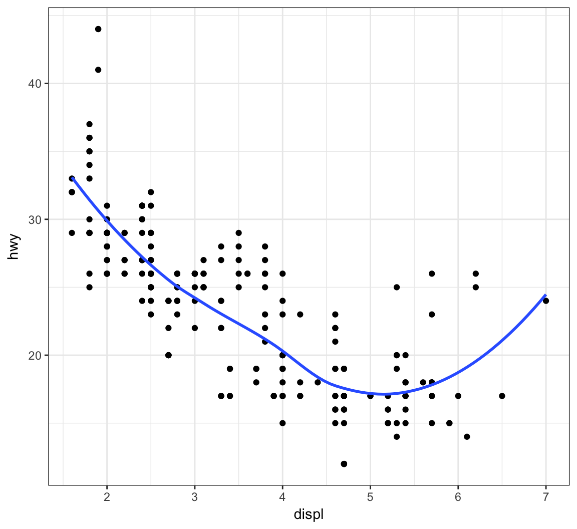
The default smoother here is a “loess” smoother. Let’s compare that to the least squares regresson line:
> ggplot(data = mpg, mapping = aes(x = displ, y = hwy)) +
+   geom_point() +
+   geom_smooth(aes(colour = "loess"), method = "loess", se = FALSE) +
+   geom_smooth(aes(colour = "lm"), method = "lm", se = FALSE)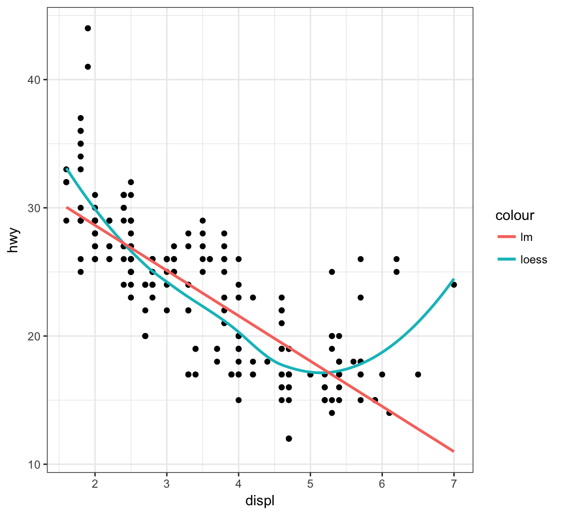
Now let’s plot a smoother to the points stratified by the drv variable:
> ggplot(data=mpg, mapping = aes(x = displ, y = hwy,
+                                linetype = drv)) +
+   geom_point() +
+   geom_smooth(se=FALSE)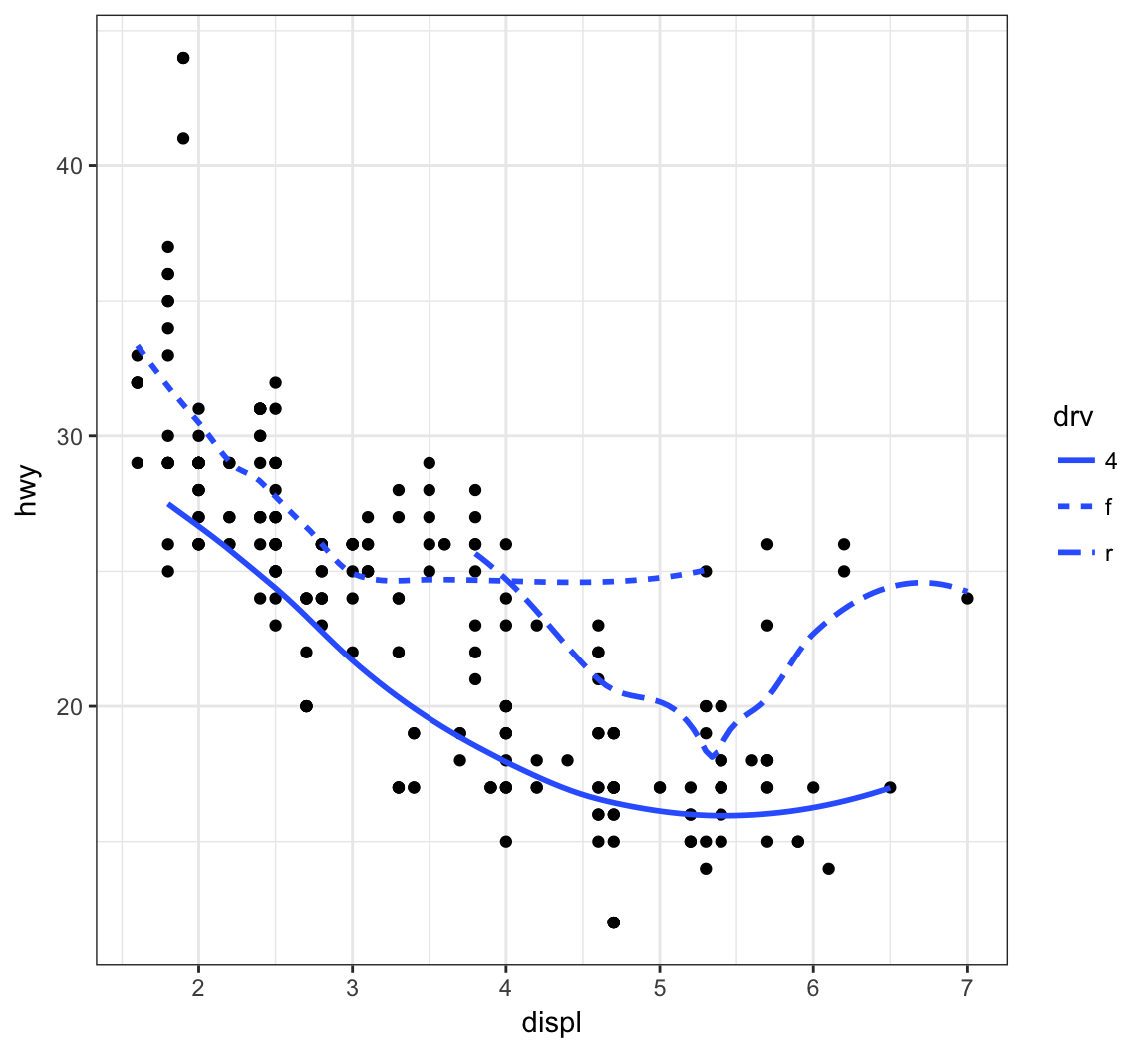
Instead of different line types, let’s instead differentiate them by line color:
> ggplot(data = mpg, mapping = aes(x = displ, y = hwy,
+                                  color=drv)) +
+   geom_point() +
+   geom_smooth(se=FALSE)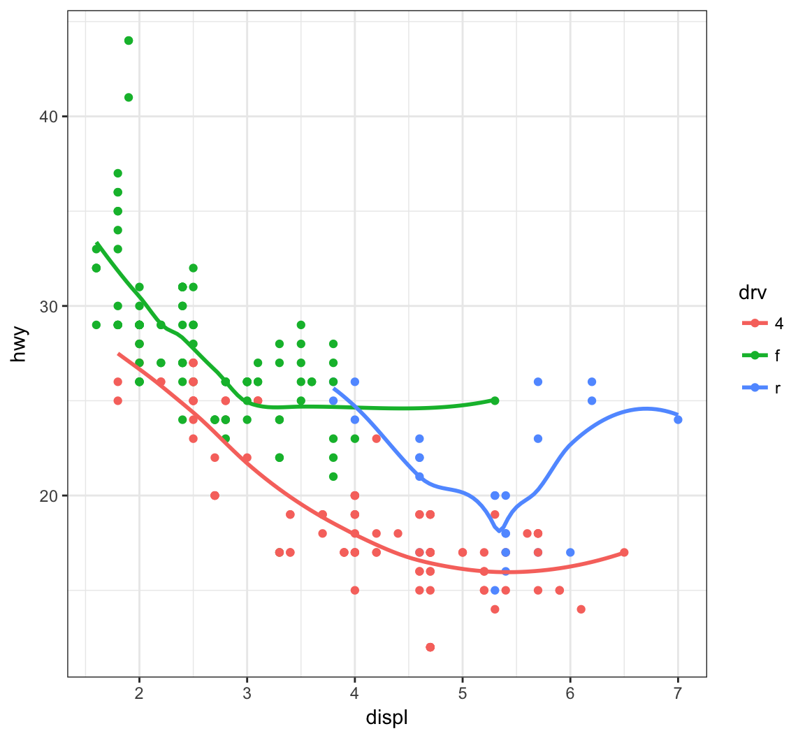
Here is an example of an overplotted scatterplot:
> ggplot(data = diamonds, mapping = aes(x=carat, y=price)) +
+   geom_point()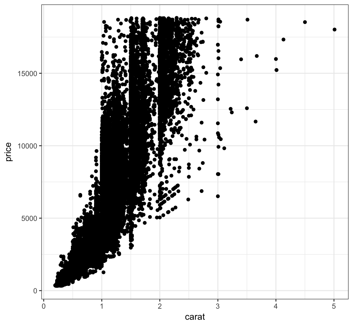
Let’s reduce the alpha of the points:
> ggplot(data = diamonds, mapping = aes(x=carat, y=price)) +
+   geom_point(alpha=0.1)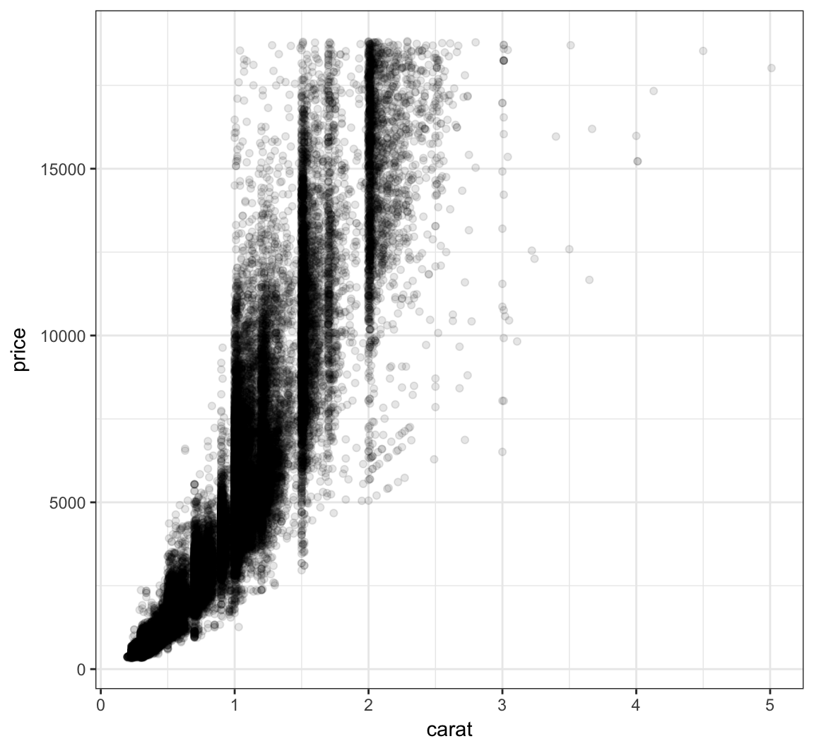
Let’s further reduce the alpha:
> ggplot(data = diamonds, mapping = aes(x=carat, y=price)) +
+   geom_point(alpha=0.01)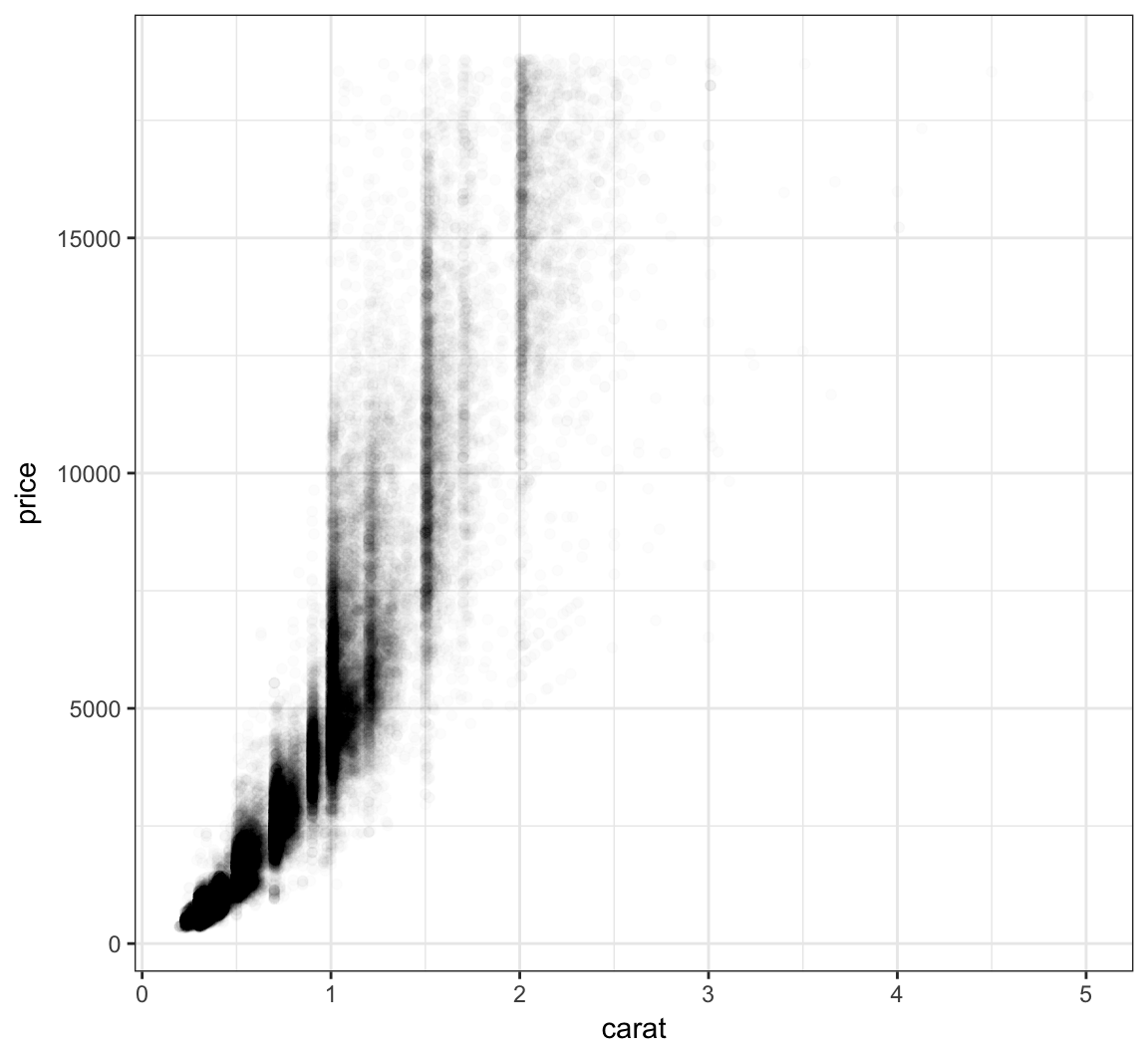
We can bin the points into hexagons, and report how many points fall within each bin. We use the geom_hex() layer to do this:
> ggplot(data = diamonds, mapping = aes(x=carat, y=price)) +
+   geom_hex()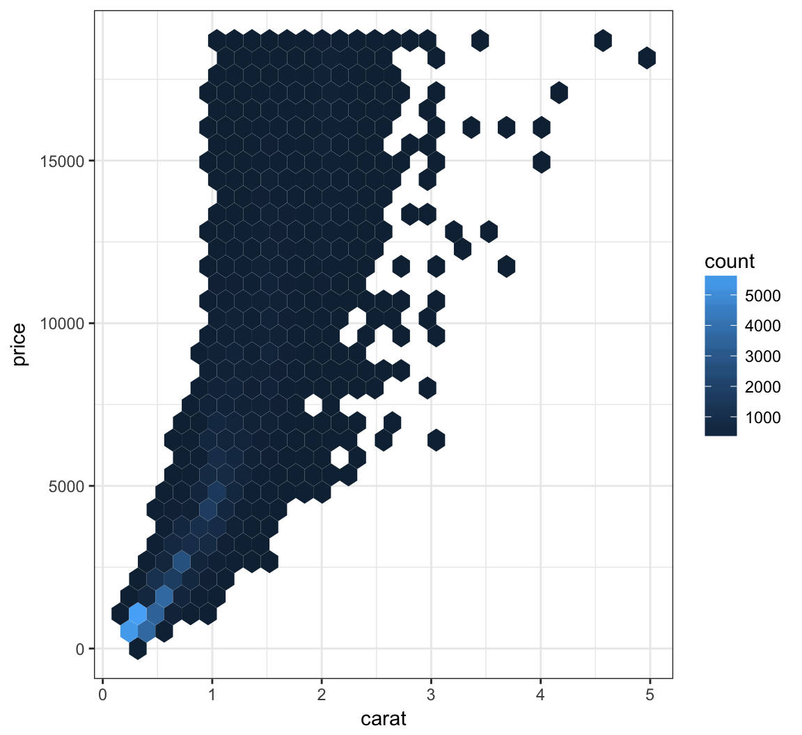
Let’s try to improve the color scheme:
> ggplot(data = diamonds, mapping = aes(x=carat, y=price)) +
+   geom_hex() +
+   scale_fill_gradient2(low="lightblue", mid="purple", high="black",
+                        midpoint=3000)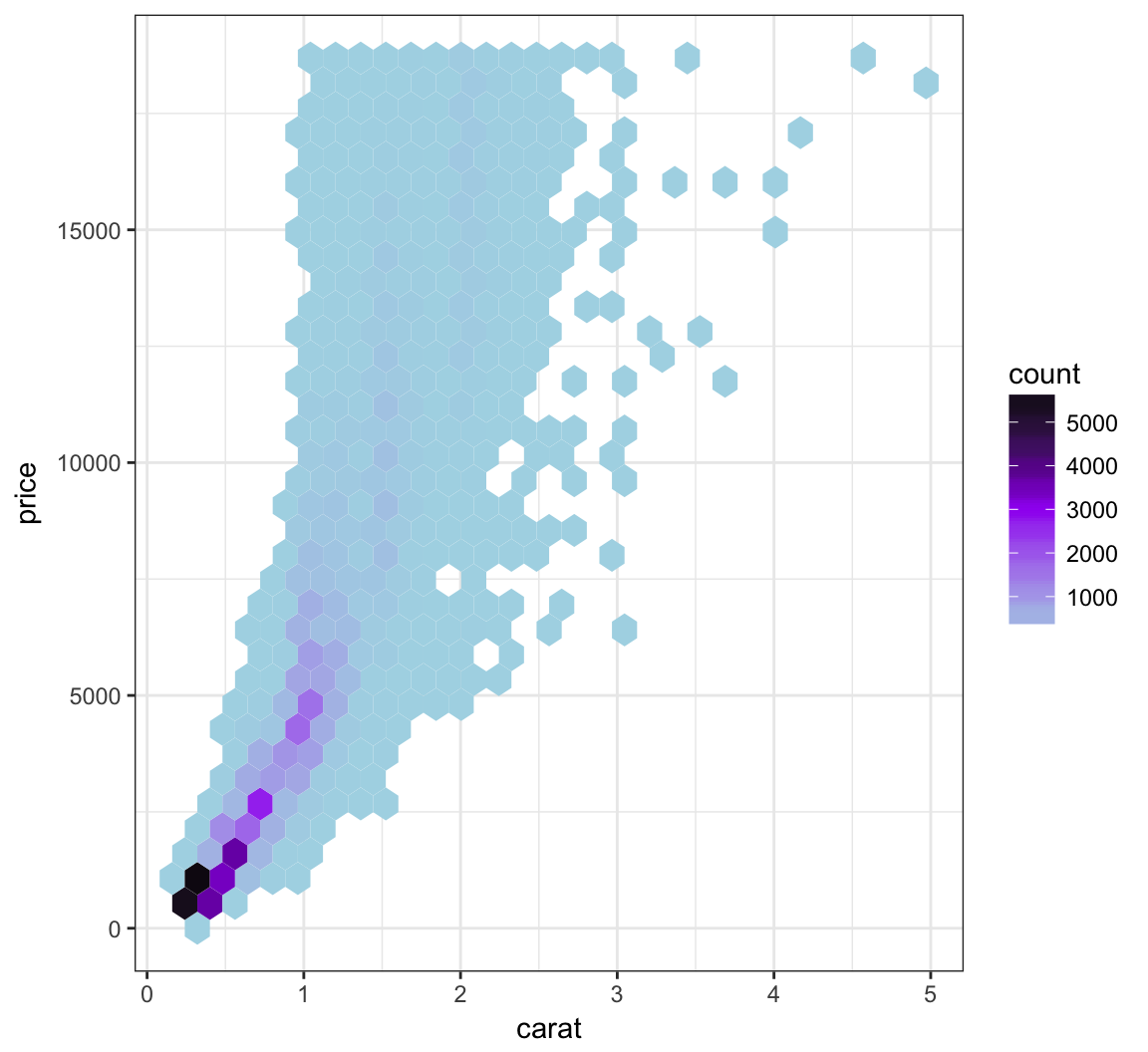
We can combine the scale transformation used earlier with the “hexbin” plotting method:
> ggplot(data = diamonds, mapping = aes(x=carat, y=price)) +
+   geom_hex(bins=20) +
+ scale_x_log10(breaks=1:5) + scale_y_log10(breaks=c(1000,5000,10000)) 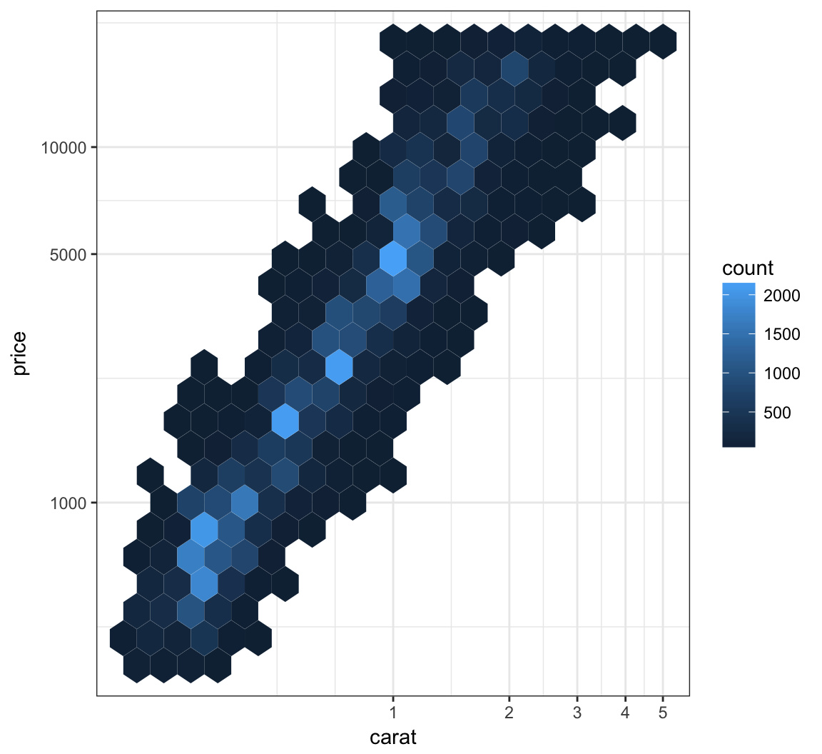
Here’s how you can change the axis labels and give the plot a title:
> ggplot(data = mpg) +
+   geom_boxplot(mapping = aes(x = factor(cyl), y = hwy)) +
+   labs(title="Highway MPG by Cylinders",x="Cylinders",
+        y="Highway MPG")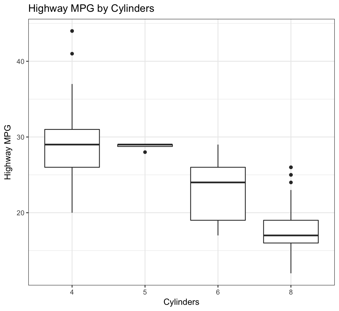
You can remove the legend to a plot by the following:
> ggplot(data = diamonds) +
+   geom_bar(mapping = aes(x = cut, fill = cut)) +
+   theme(legend.position="none")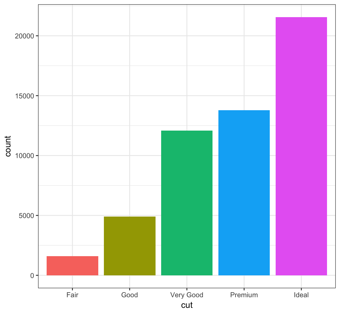
The legend can be placed on the “top”, “bottom”, “left”, or “right”:
> ggplot(data = diamonds) +
+   geom_bar(mapping = aes(x = cut, fill = cut)) +
+   theme(legend.position="bottom")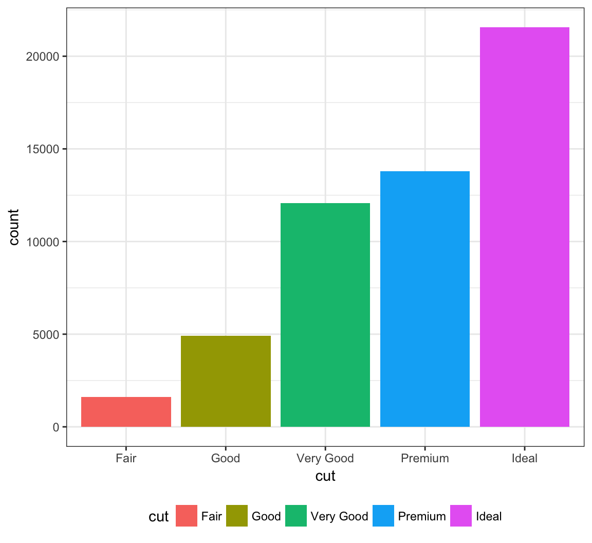
The legend can be moved inside the plot itself:
> ggplot(data = diamonds) +
+   geom_bar(mapping = aes(x = cut, fill = cut)) +
+   theme(legend.position=c(0.15,0.75))
Change the name of the legend:
> ggplot(data = diamonds) +
+   geom_bar(mapping = aes(x = cut, fill = cut)) +
+   scale_fill_discrete(name="Diamond\nCut")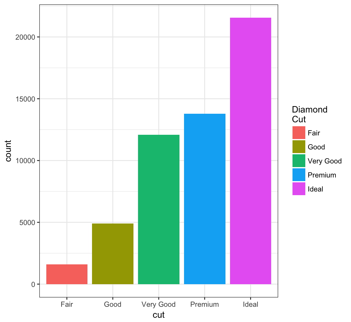
Change the labels within the legend:
> ggplot(data = diamonds) +
+   geom_bar(mapping = aes(x = cut, fill = cut)) +
+   scale_fill_discrete(labels=c("F", "G", "VG", "P", "I"))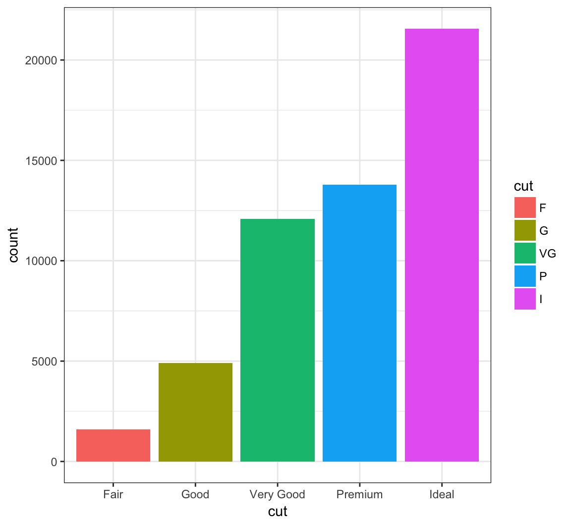
Here is the histogram of the displ variable from the mpg data set:
> ggplot(mpg) + geom_histogram(mapping=aes(x=displ),
+                              binwidth=0.25)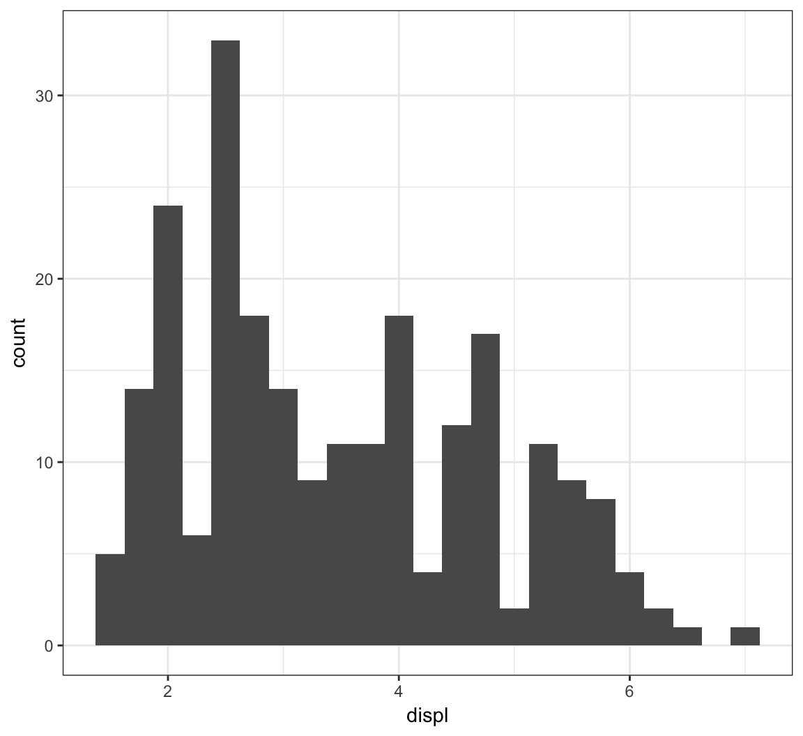
The facet_wrap() layer allows us to stratify the displ variable according to cyl, and show the histograms for the strata in an organized fashion:
> ggplot(mpg) +
+   geom_histogram(mapping=aes(x=displ), binwidth=0.25) +
+   facet_wrap(~ cyl)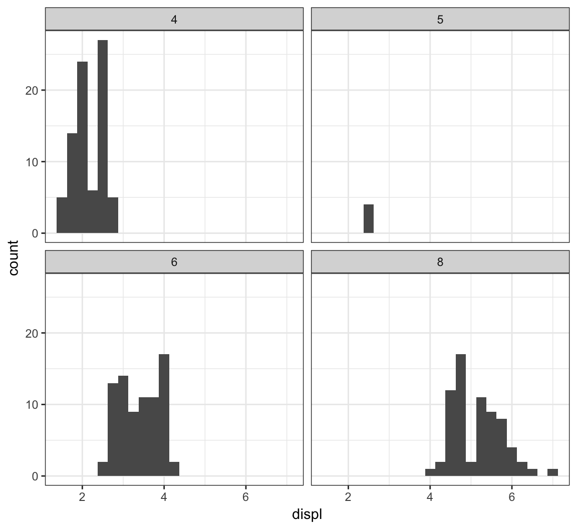
Here is facet_wrap() applied to displ startified by the drv variable:
> ggplot(mpg) +
+   geom_histogram(mapping=aes(x=displ), binwidth=0.25) +
+   facet_wrap(~ drv)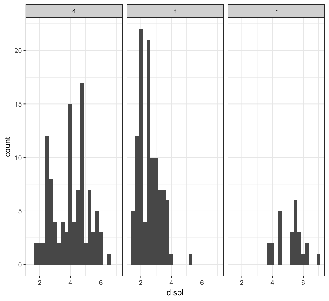
We can stratify by two variable simultaneously by using the facet_grid() layer:
> ggplot(mpg) +
+   geom_histogram(mapping=aes(x=displ), binwidth=0.25) +
+   facet_grid(drv ~ cyl)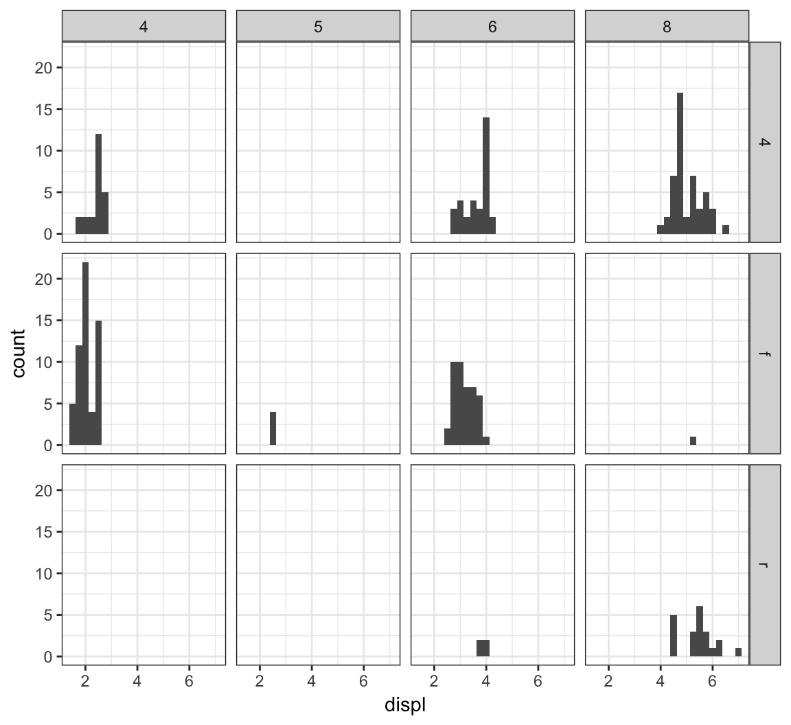
Let’s carry out a similar faceting on the diamonds data over the next four plots:
> ggplot(diamonds) +
+   geom_histogram(mapping=aes(x=price), binwidth=500)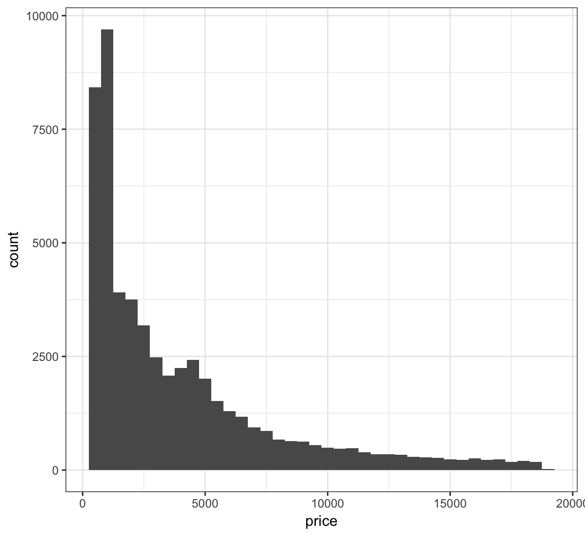
Stratify price by clarity:
> ggplot(diamonds) +
+   geom_histogram(mapping=aes(x=price), binwidth=500) +
+   facet_wrap(~ clarity)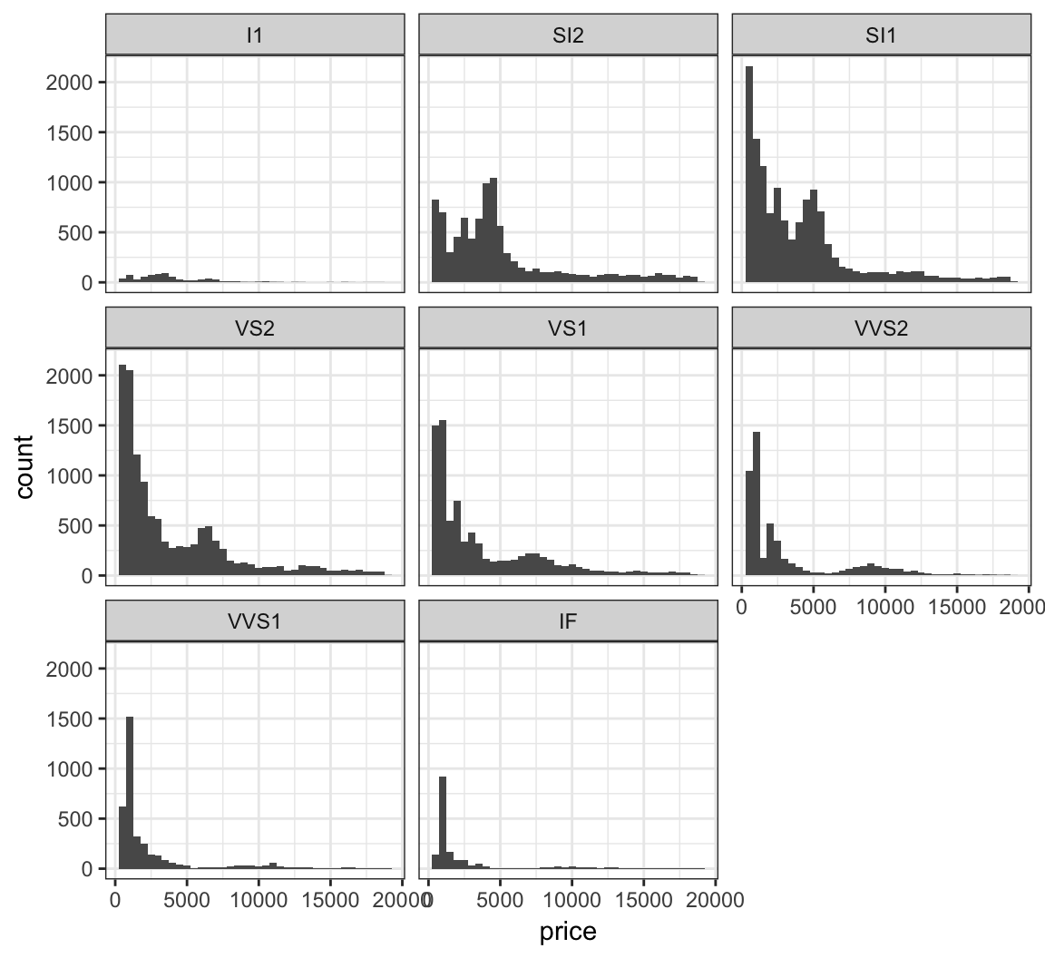
Stratify price by clarity, but allow each y-axis range to be different by including the scale="free_y" argument:
> ggplot(diamonds) +
+   geom_histogram(mapping=aes(x=price), binwidth=500) +
+   facet_wrap(~ clarity, scale="free_y")
Jointly stratify price by cut and clarify:
> ggplot(diamonds) +
+   geom_histogram(mapping=aes(x=price), binwidth=500) +
+   facet_grid(cut ~ clarity) +
+   scale_x_continuous(breaks=9000)
Manually determine colors to fill the barplot using the color blind palette defined above, cbPalette:
> ggplot(data = diamonds) +
+   geom_bar(mapping = aes(x = cut, fill = cut)) +
+   scale_fill_manual(values=cbPalette)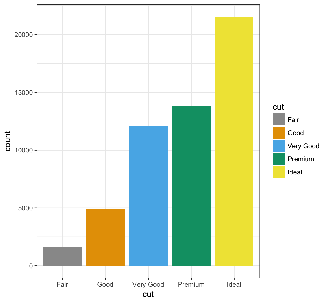
Manually determine point colors using the color blind palette defined above, cbPalette:
> ggplot(data = mpg) +
+   geom_point(mapping = aes(x = displ, y = hwy, color = class), size=2) +
+   scale_color_manual(values=cbPalette)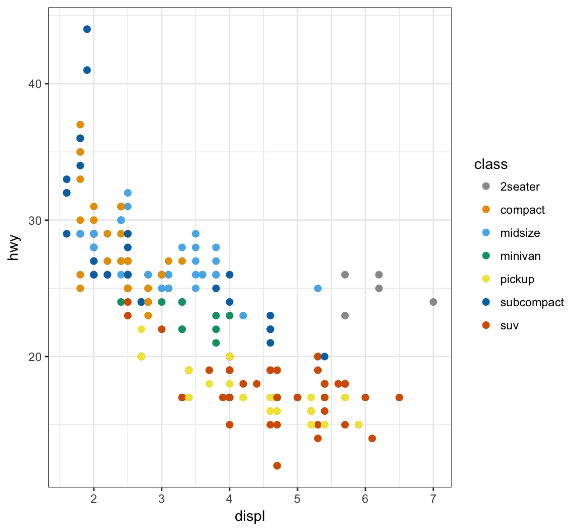
Fill the histogram bars using a color gradient by their counts, where we determine the endpoint colors:
> ggplot(data = mpg) +
+   geom_histogram(aes(x=hwy, fill=..count..)) +
+   scale_fill_gradient(low="blue", high="red")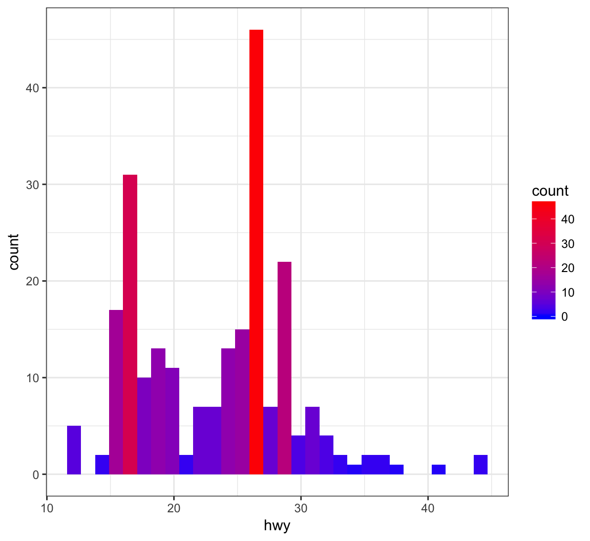
Color the points based on a gradient formed from the quantitative variable, displ, where we we determine the endpoint colors:
> ggplot(data = mpg) +
+   geom_point(aes(x=hwy, y=cty, color=displ), size=2) +
+   scale_color_gradient(low="blue", high="red")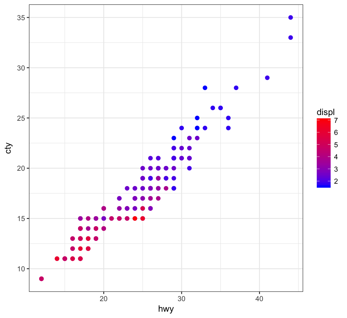
An example of using the palette “Set1” from the RColorBrewer package, included in ggplot2:
> ggplot(diamonds) +
+   geom_density(mapping = aes(x=price, color=clarity)) +
+   scale_color_brewer(palette = "Set1")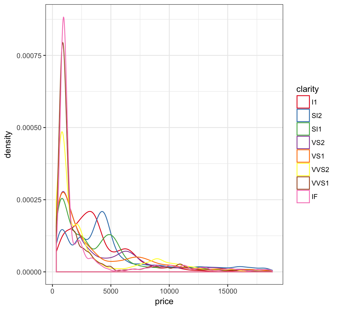
Another example of using the palette “Set1” from the RColorBrewer package, included in ggplot2:
> ggplot(data = mpg) +
+   geom_point(mapping = aes(x = displ, y = hwy, color = class)) +
+   scale_color_brewer(palette = "Set1")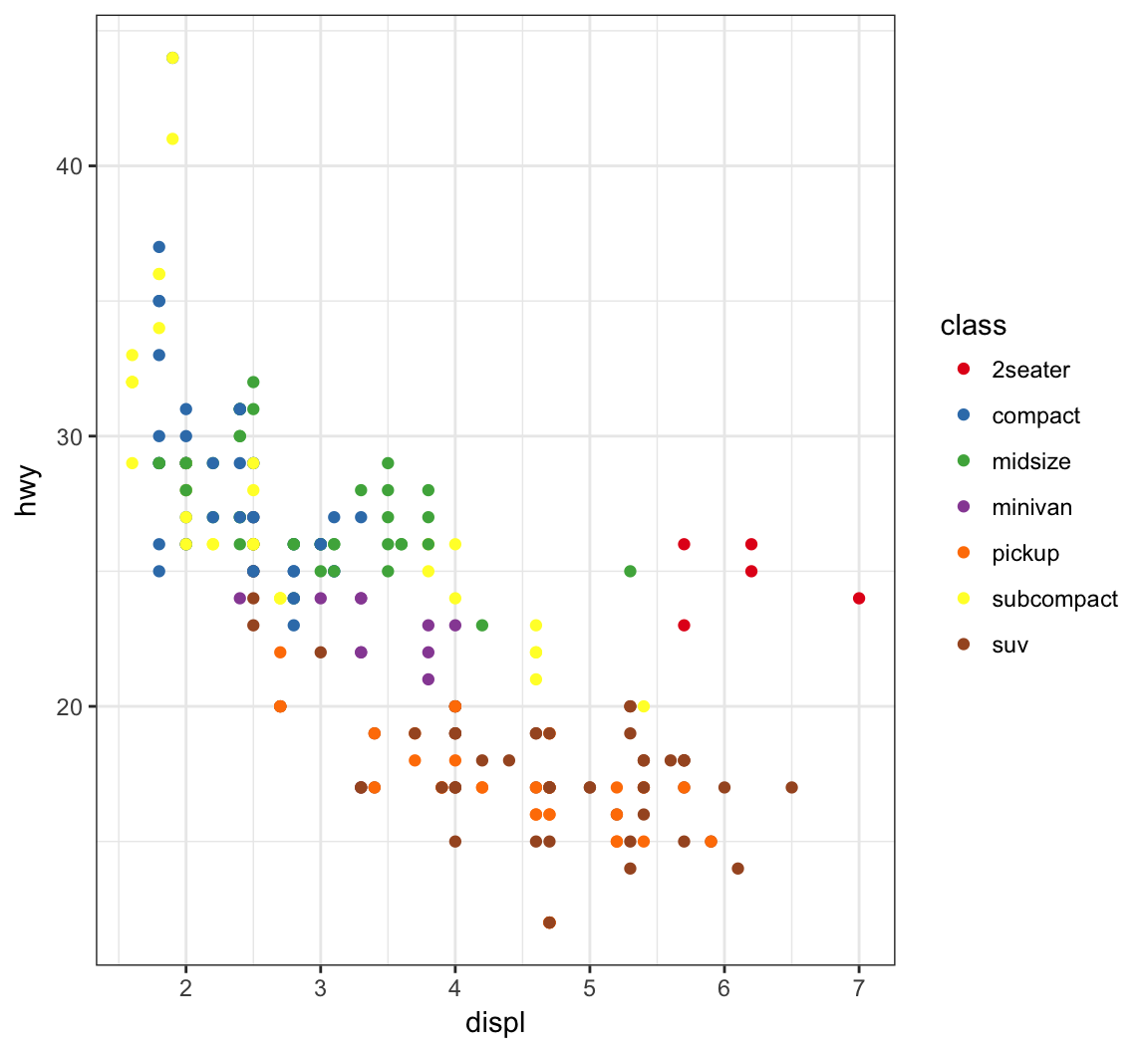
The gapminder package comes with its own set of colors, country_colors.
> ggplot(subset(gapminder, continent != "Oceania"),
+        aes(x = year, y = lifeExp, group = country,
+            color = country)) +
+   geom_line(show.legend = FALSE) + facet_wrap(~ continent) +
+   scale_color_manual(values = country_colors)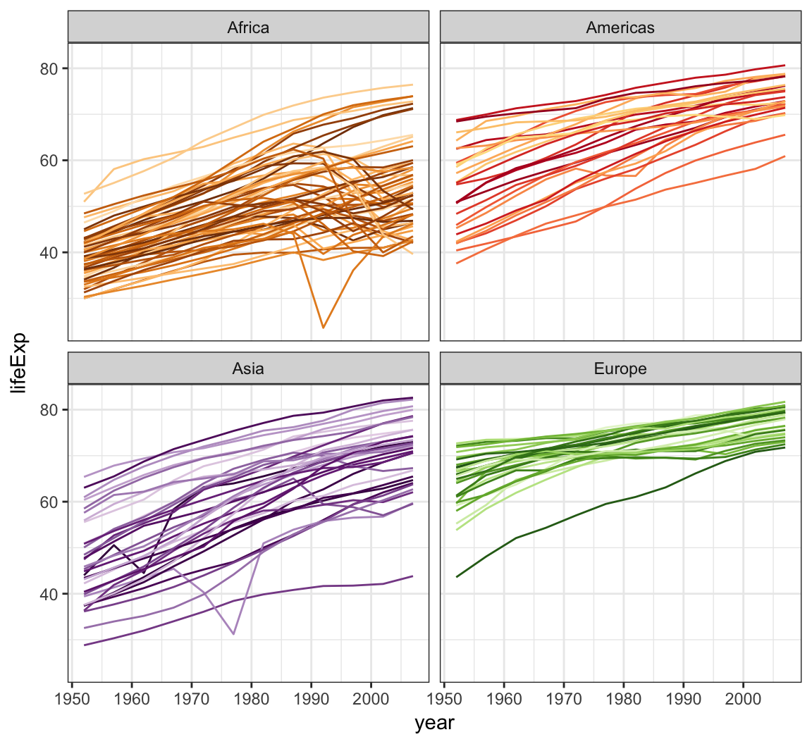
Available Themes
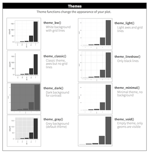
From http://r4ds.had.co.nz/visualize.html. See also ggthemes package.
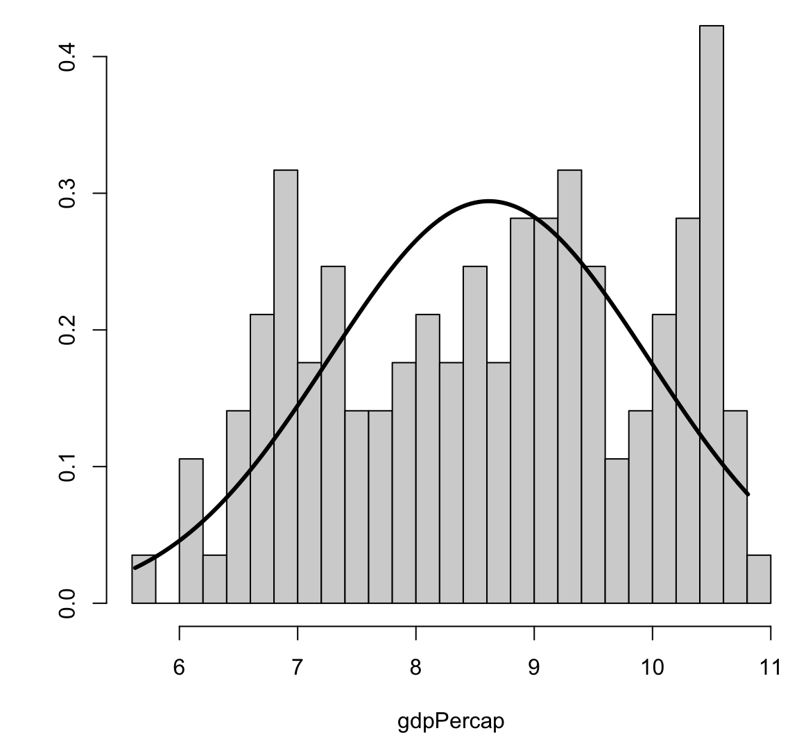
Visualizing Skewness and Kurtosis
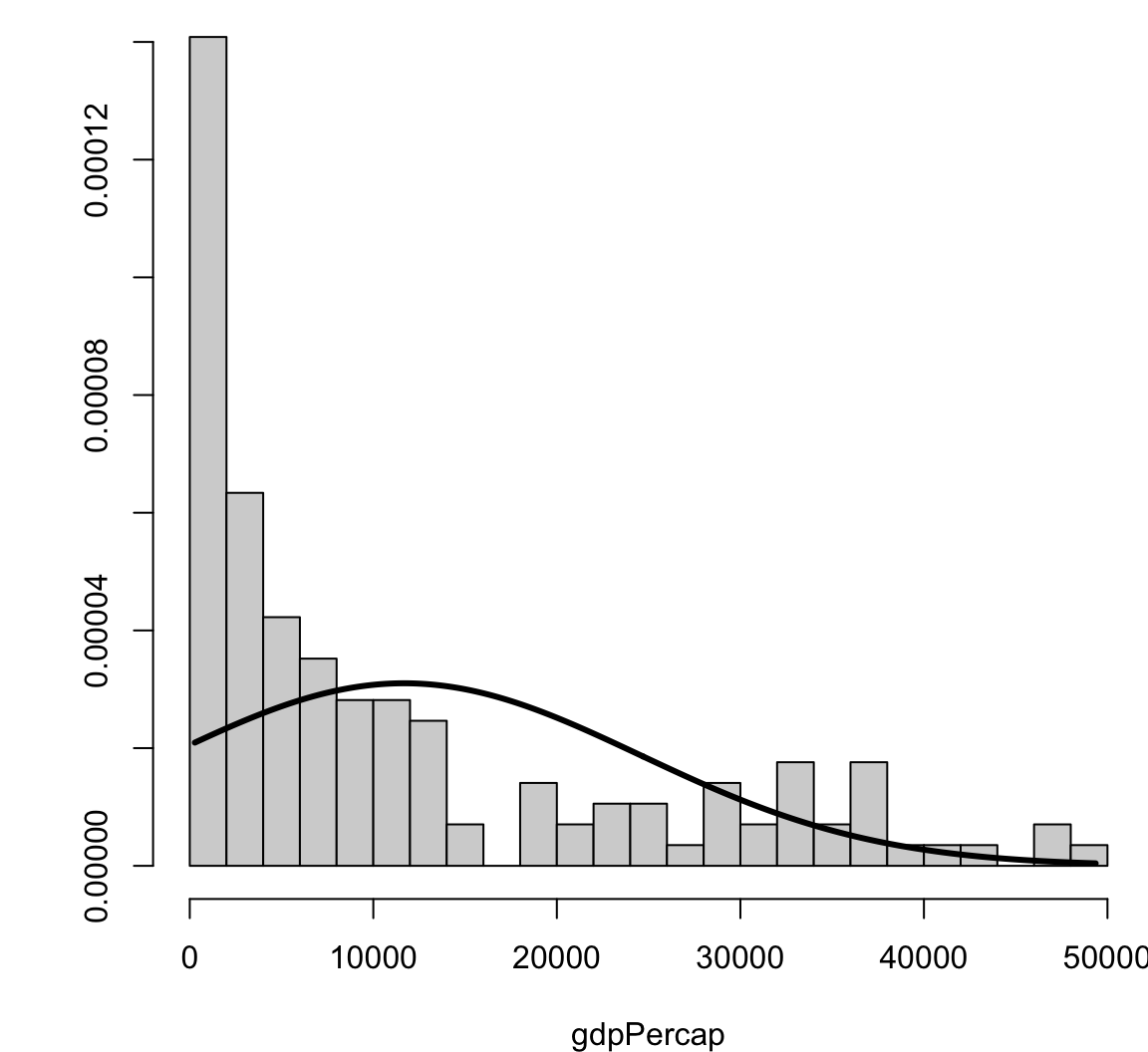
Visualizing Skewness and Kurtosis
> x <- rnorm(500)
> y <- x + rnorm(500)
> cor(x, y, method="pearson")
[1] 0.7542651
> cor(x, y, method="spearman")
[1] 0.7499555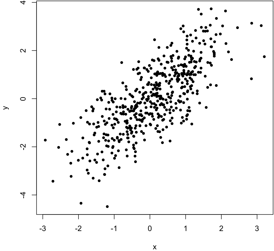
> x <- rnorm(500)
> y <- x + rnorm(500, sd=2)
> cor(x, y, method="pearson")
[1] 0.5164903
> cor(x, y, method="spearman")
[1] 0.5093092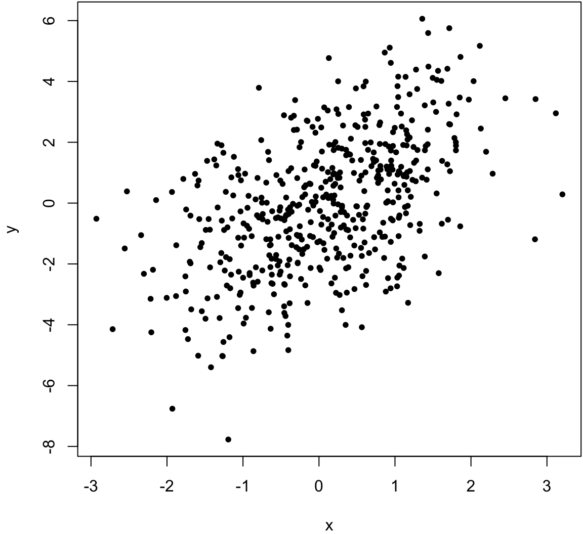
> x <- c(rnorm(499), 100)
> y <- c(rnorm(499), 100)
> cor(x, y, method="pearson")
[1] 0.9528564
> cor(x, y, method="spearman")
[1] -0.02133551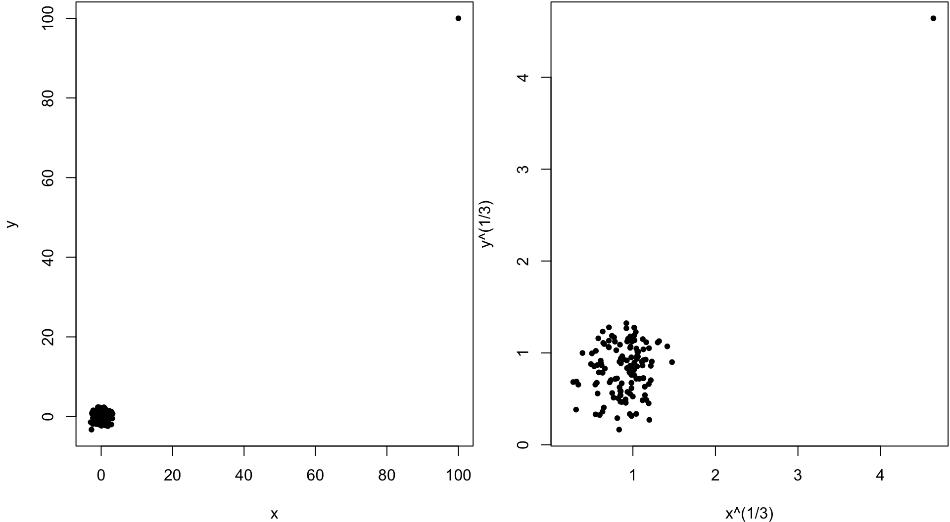
> qqnorm(mtcars$mpg, main=" ")
> qqline(mtcars$mpg) # line through Q1 and Q3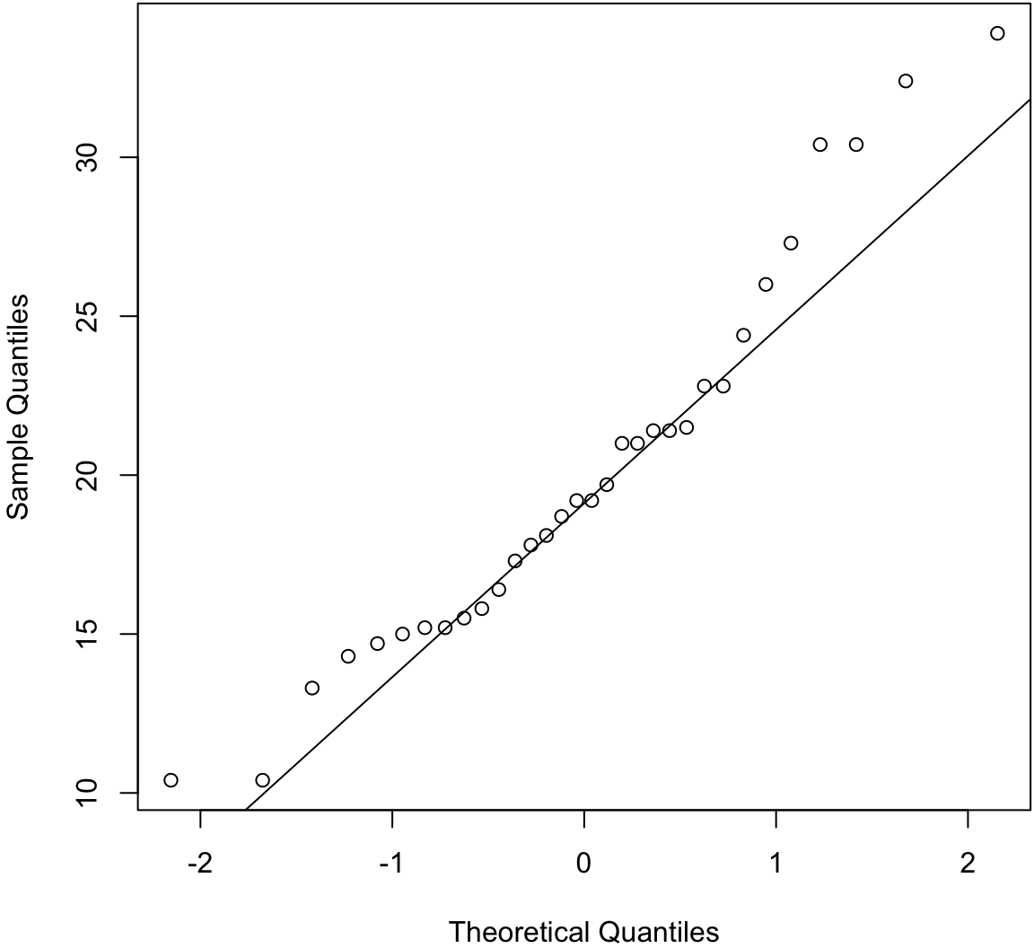
> before1980 <- gapminder %>% filter(year < 1980) %>%
+   select(lifeExp) %>% unlist()
> after1980 <- gapminder %>% filter(year > 1980) %>%
+   select(lifeExp) %>% unlist()
> qqplot(before1980, after1980); abline(0,1)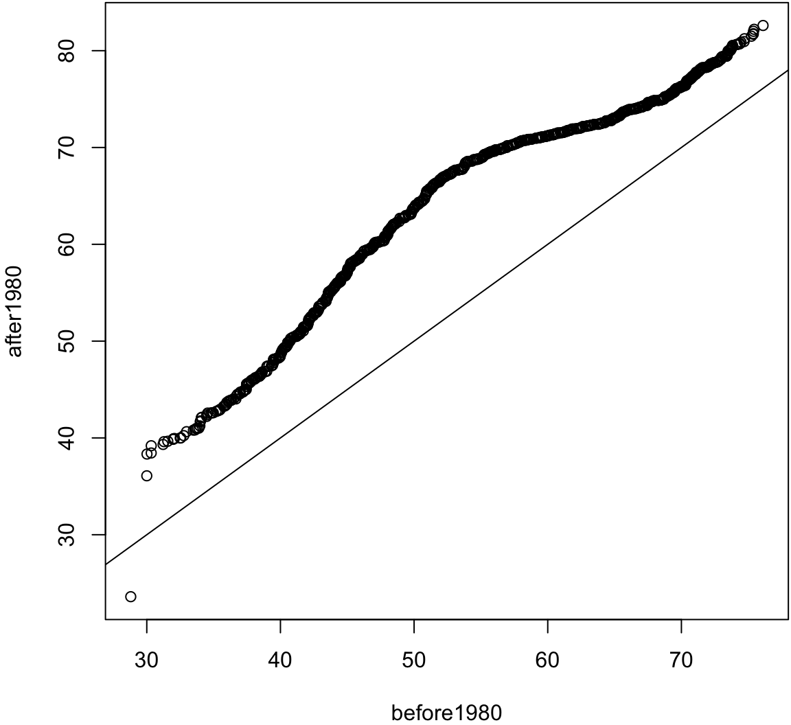
> ggplot(mtcars) + stat_qq(aes(sample = mpg))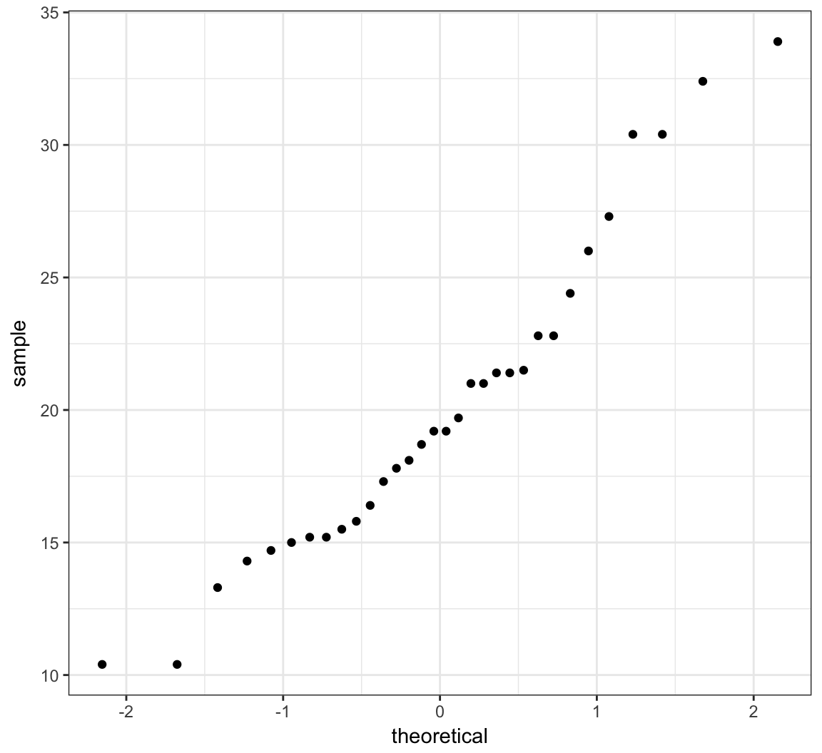
> ggplot(gapminder) + stat_qq(aes(sample=lifeExp))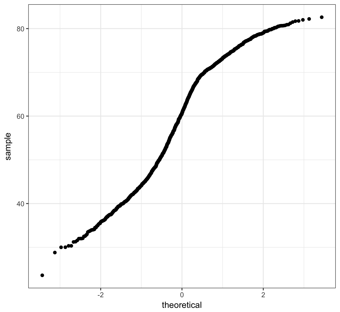
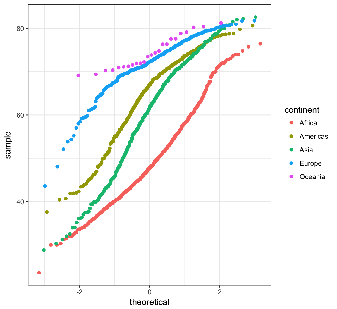
> ggplot(gapminder) +
+   stat_qq(aes(sample=lifeExp, color=continent))