QCB 508 – Week 2

John D. Storey

Spring 2017

Data Wrangling

Definition

Data wrangling is loosely defined as the process of manually converting or mapping data from one “raw” form into another format that allows for more convenient consumption of the data with the help of semi-automated tools.

It typically follows a set of general steps which begin with extracting the data in a raw form from the data source, “wrangling” the raw data using algorithms (e.g. sorting) or parsing the data into predefined data structures, and finally depositing the resulting content into a data sink for storage and future use.

From https://en.wikipedia.org/wiki/Data_wrangling

Workflow

These steps are typically taken in a data science project.

Import
Tidy
Transform \(\leftrightarrow\) Visualize \(\leftrightarrow\) Model (iterate)
Communicate

The bold terms are part of data wrangling.

Challenges

Importing files
Organizing data sets
Transforming data
Combining data sets
Dealing with various data types (e.g., dates)
Identifying errors

Tidy Data

Motivation

“Happy families are all alike; every unhappy family is unhappy in its own way.” – Leo Tolstoy

“Tidy datasets are all alike, but every messy dataset is messy in its own way.” – Hadley Wickham

From R for Data Science.

Definition

Tidy datasets are easy to manipulate, model and visualize, and have a specific structure: each variable is a column, each observation is a row, and each type of observational unit is a table.

From Wickham (2014), “Tidy Data”, Journal of Statistical Software

A dataset is a collection of values, usually either numbers (if quantitative) or strings (if qualitative). Values are organized in two ways. Every value belongs to a variable and an observation. A variable contains all values that measure the same underlying attribute (like height, temperature, duration) across units. An observation contains all values measured on the same unit (like a person, or a day, or a race) across attributes.

From: Wickham H (2014), “Tidy Data”, Journal of Statistical Software

Example: Titanic Data

According to the Titanic data from the datasets package: 367 males survived, 1364 males perished, 344 females survived, and 126 females perished.

How should we organize these data?

Intuitive Format

	Survived	Perished
Male	367	1364
Female	344	126

Tidy Format

fate	sex	number
perished	male	1364
perished	female	126
survived	male	367
survived	female	344

Rules of Thumb

Something is a value if it represents different forms of a common object and it changes throughout the data set.
Something is a value if the data can be arranged so that it appears across rows within a column and this makes sense.

For example, fate and sex do not satisfy these criteria in the Titanic data, but perished/survived and female/male do.

Tidyverse

Idea

When the data are in tidy format, one can design functions around this format to consistently and intuitively perform data wrangling and analysis operations. The packages containing these are called the “tidyverse.”

Note: The idea of tidy data was first proposed by Hadley Wickham and he created several of the core packages, so this used to be called (semi-seriously) the “hadleyverse.”

Packages

The tidyverse is a set of packages that work in harmony because they share common data representations and API design. The tidyverse package is designed to make it easy to install and load core packages from the tidyverse in a single command.

https://blog.rstudio.org/2016/09/15/tidyverse-1-0-0/

Primary Packages

dplyr: data manipulation
ggplot2: data visualization
purrr: functional programming
readr: data import
tibble: modernization of data frames
tidyr: data tidying

Loading `tidyverse`

> library(tidyverse)

Tidying Data

`tidyr` Package

This package provides a variety of functions that allow one to tidy data.

Importantly, it solves two common ways that data come as untidy.

gather(): Gathers a variable distributed across two or more columns into a single column.
spread(): Spreads a column containing two or more variables into one column per variable.

Untidy Titanic Data

This does not satisfy the definition of tidy data because a variable’s observations are distributed as column names.

> df <- tibble(sex=c("male", "female"), 
+              survived=c(367, 344),
+              perished=c(1364, 126))
> df
# A tibble: 2 × 3
     sex survived perished
   <chr>    <dbl>    <dbl>
1   male      367     1364
2 female      344      126

`gather()`

We apply the gather() function to make a column containing the survived and perished observations.

> df <- gather(df, survived, perished, 
+                key="fate", value="number")
> df
# A tibble: 4 × 3
     sex     fate number
   <chr>    <chr>  <dbl>
1   male survived    367
2 female survived    344
3   male perished   1364
4 female perished    126

`spread()`

This example is here to show that spread() does the opposite operation as gather(). It isn’t used appropriately here because we revert the data back to untidy format.

> spread(df, key=fate, value=number)
# A tibble: 2 × 3
     sex perished survived
*  <chr>    <dbl>    <dbl>
1 female      126      344
2   male     1364      367

Tidy with `spread()`

Median cost of home and median income per city are two variables included in a single column. This means we need to use spread().

> df
# A tibble: 4 × 3
     city median_value dollars
    <chr>        <chr>   <dbl>
1  Boston         home  527300
2  Boston       income   71738
3 Raleigh         home  215700
4 Raleigh       income   65778

> spread(df, key=median_value, value=dollars)
# A tibble: 2 × 3
     city   home income
*   <chr>  <dbl>  <dbl>
1  Boston 527300  71738
2 Raleigh 215700  65778

Reshaping Data

Wide vs. Long Format

Tidy data are in “wide format” in that they have a column for each variable and there is one observed unit per row.

However, sometimes it’s useful to transform to “long format.” The simplest long format data have two columns. The first column contains the variable names and the second colum contains the values for the variables. There are “wider” long format data that have additional columns that identify connections between observations.

Wide format data is useful for some analyses and long format for others.

`reshape2` Package

The reshape2 package has three important functions: melt, dcast, and acast. It allows one to move between wide and long tidy data formats.

> library("reshape2")
> library("datasets")
> data(airquality, package="datasets")
> names(airquality)
[1] "Ozone"   "Solar.R" "Wind"    "Temp"    "Month"   "Day"    
> dim(airquality)
[1] 153   6
> airquality <- as_tibble(airquality)

Air Quality Data Set

> head(airquality)
# A tibble: 6 × 6
  Ozone Solar.R  Wind  Temp Month   Day
  <int>   <int> <dbl> <int> <int> <int>
1    41     190   7.4    67     5     1
2    36     118   8.0    72     5     2
3    12     149  12.6    74     5     3
4    18     313  11.5    62     5     4
5    NA      NA  14.3    56     5     5
6    28      NA  14.9    66     5     6

> tail(airquality)
# A tibble: 6 × 6
  Ozone Solar.R  Wind  Temp Month   Day
  <int>   <int> <dbl> <int> <int> <int>
1    14      20  16.6    63     9    25
2    30     193   6.9    70     9    26
3    NA     145  13.2    77     9    27
4    14     191  14.3    75     9    28
5    18     131   8.0    76     9    29
6    20     223  11.5    68     9    30

Melt

Melting can be thought of as melting a piece of solid metal (wide data), so it drips into long format.

> aql <- melt(airquality)
No id variables; using all as measure variables
> head(aql)
  variable value
1    Ozone    41
2    Ozone    36
3    Ozone    12
4    Ozone    18
5    Ozone    NA
6    Ozone    28

> tail(aql)
    variable value
913      Day    25
914      Day    26
915      Day    27
916      Day    28
917      Day    29
918      Day    30

Guided Melt

In the previous example, we lose the fact that a set of measurements occurred on a particular day and month, so we can do a guided melt to keep this information.

> aql <- melt(airquality, id.vars = c("Month", "Day"))
> head(aql)
  Month Day variable value
1     5   1    Ozone    41
2     5   2    Ozone    36
3     5   3    Ozone    12
4     5   4    Ozone    18
5     5   5    Ozone    NA
6     5   6    Ozone    28

> tail(aql)
    Month Day variable value
607     9  25     Temp    63
608     9  26     Temp    70
609     9  27     Temp    77
610     9  28     Temp    75
611     9  29     Temp    76
612     9  30     Temp    68

Casting

Casting allows us to go from long format to wide format data. It can be visualized as pouring molten metal (long format) into a cast to create a solid piece of metal (wide format).

Casting is more difficult because choices have to be made to determine how the wide format will be organized. It often takes some thought and experimentation for new users.

Let’s do an example with dcast, which is casting for data frames.

`dcast()`

> aqw <- dcast(aql, Month + Day ~ variable)
> head(aqw)
  Month Day Ozone Solar.R Wind Temp
1     5   1    41     190  7.4   67
2     5   2    36     118  8.0   72
3     5   3    12     149 12.6   74
4     5   4    18     313 11.5   62
5     5   5    NA      NA 14.3   56
6     5   6    28      NA 14.9   66

> tail(aqw)
    Month Day Ozone Solar.R Wind Temp
148     9  25    14      20 16.6   63
149     9  26    30     193  6.9   70
150     9  27    NA     145 13.2   77
151     9  28    14     191 14.3   75
152     9  29    18     131  8.0   76
153     9  30    20     223 11.5   68

Transforming Data

`dplyr` Package

dplyr is a package with the following description:

A fast, consistent tool for working with data frame like objects, both in memory and out of memory.

This package offers a “grammar” for manipulating data frames.

Everything that dplyr does can also be done using basic R commands – however, it tends to be much faster and easier to use dplyr.

Grammar of `dplyr`

Verbs:

filter: extract a subset of rows from a data frame based on logical conditions
arrange: reorder rows of a data frame
rename: rename variables in a data frame
select: return a subset of the columns of a data frame, using a flexible notation

mutate: add new variables/columns or transform existing variables
distinct: returns only the unique values in a table
summarize: generate summary statistics of different variables in the data frame, possibly within strata
group_by: breaks down a dataset into specified groups of rows

Partially based on R Programming for Data Science

Example: Baby Names

> library("dplyr", verbose=FALSE)
> library("babynames")
> ls()
character(0)
> babynames <- as_tibble(babynames::babynames)
> ls()
[1] "babynames"

`babynames` Object

> class(babynames)
[1] "tbl_df"     "tbl"        "data.frame"
> dim(babynames)
[1] 1858689       5

> babynames
# A tibble: 1,858,689 × 5
    year   sex      name     n       prop
   <dbl> <chr>     <chr> <int>      <dbl>
1   1880     F      Mary  7065 0.07238433
2   1880     F      Anna  2604 0.02667923
3   1880     F      Emma  2003 0.02052170
4   1880     F Elizabeth  1939 0.01986599
5   1880     F    Minnie  1746 0.01788861
6   1880     F  Margaret  1578 0.01616737
7   1880     F       Ida  1472 0.01508135
8   1880     F     Alice  1414 0.01448711
9   1880     F    Bertha  1320 0.01352404
10  1880     F     Sarah  1288 0.01319618
# ... with 1,858,679 more rows

Peek at the Data

> set.seed(201)
> sample_n(babynames, 10) 
# A tibble: 10 × 5
    year   sex     name     n         prop
   <dbl> <chr>    <chr> <int>        <dbl>
1   1992     M   Kelcey    17 8.101322e-06
2   1933     M   Hervey    14 1.372698e-05
3   1968     M     Rich   116 6.529976e-05
4   1906     F    Annis    30 9.571179e-05
5   1993     M Stefanos     9 4.358763e-06
6   1928     F   Janine    10 8.365506e-06
7   1908     M    Pedro    53 3.185632e-04
8   1968     M Rosemary     6 3.377574e-06
9   1921     F    Rheda     7 5.470113e-06
10  1956     M Clemente    26 1.212302e-05
> # try also sample_frac(babynames, 6e-6)

`%>%` Operator

Originally from R package magrittr. Provides a mechanism for chaining commands with a forward-pipe operator, %>%.

> x <- 1:10
> 
> x %>% log(base=10) %>% sum
[1] 6.559763
> 
> sum(log(x,base=10))
[1] 6.559763

> babynames %>% sample_n(5)
# A tibble: 5 × 5
   year   sex      name     n         prop
  <dbl> <chr>     <chr> <int>        <dbl>
1  1980     F      Pola     6 3.370355e-06
2  1997     F Shermaine     8 4.191640e-06
3  1992     F       Mee    17 8.482331e-06
4  1980     M     Abram   147 7.925844e-05
5  1985     F   Coralia     6 3.250954e-06

`filter()`

> filter(babynames, year==1880, sex=="F")
# A tibble: 942 × 5
    year   sex      name     n       prop
   <dbl> <chr>     <chr> <int>      <dbl>
1   1880     F      Mary  7065 0.07238433
2   1880     F      Anna  2604 0.02667923
3   1880     F      Emma  2003 0.02052170
4   1880     F Elizabeth  1939 0.01986599
5   1880     F    Minnie  1746 0.01788861
6   1880     F  Margaret  1578 0.01616737
7   1880     F       Ida  1472 0.01508135
8   1880     F     Alice  1414 0.01448711
9   1880     F    Bertha  1320 0.01352404
10  1880     F     Sarah  1288 0.01319618
# ... with 932 more rows
> # same as filter(babynames, year==1880 & sex=="F")

> filter(babynames, year==1880, sex=="F", n > 5000)
# A tibble: 1 × 5
   year   sex  name     n       prop
  <dbl> <chr> <chr> <int>      <dbl>
1  1880     F  Mary  7065 0.07238433

`arrange()`

> arrange(babynames, name, year, sex)
# A tibble: 1,858,689 × 5
    year   sex  name     n         prop
   <dbl> <chr> <chr> <int>        <dbl>
1   2007     M Aaban     5 2.259872e-06
2   2009     M Aaban     6 2.833201e-06
3   2010     M Aaban     9 4.388578e-06
4   2011     M Aaban    11 5.427020e-06
5   2012     M Aaban    11 5.435940e-06
6   2013     M Aaban    14 6.952863e-06
7   2014     M Aaban    16 7.843929e-06
8   2015     M Aaban    15 7.400566e-06
9   2011     F Aabha     7 3.620673e-06
10  2012     F Aabha     5 2.585247e-06
# ... with 1,858,679 more rows

`arrange()`

> arrange(babynames, desc(name), desc(year), sex)
# A tibble: 1,858,689 × 5
    year   sex      name     n         prop
   <dbl> <chr>     <chr> <int>        <dbl>
1   2010     M     Zzyzx     5 2.438099e-06
2   2014     M     Zyyon     6 2.941474e-06
3   2010     F   Zyyanna     6 3.066148e-06
4   2015     M     Zyvon     6 2.960226e-06
5   2009     M    Zyvion     5 2.361001e-06
6   2015     M      Zyus     5 2.466855e-06
7   2010     M Zytavious     6 2.925719e-06
8   2009     M Zytavious     7 3.305401e-06
9   2007     M Zytavious     6 2.711846e-06
10  2006     M Zytavious     7 3.196251e-06
# ... with 1,858,679 more rows

`rename()`

> rename(babynames, number=n)
# A tibble: 1,858,689 × 5
    year   sex      name number       prop
   <dbl> <chr>     <chr>  <int>      <dbl>
1   1880     F      Mary   7065 0.07238433
2   1880     F      Anna   2604 0.02667923
3   1880     F      Emma   2003 0.02052170
4   1880     F Elizabeth   1939 0.01986599
5   1880     F    Minnie   1746 0.01788861
6   1880     F  Margaret   1578 0.01616737
7   1880     F       Ida   1472 0.01508135
8   1880     F     Alice   1414 0.01448711
9   1880     F    Bertha   1320 0.01352404
10  1880     F     Sarah   1288 0.01319618
# ... with 1,858,679 more rows

`select()`

> select(babynames, sex, name, n)
# A tibble: 1,858,689 × 3
     sex      name     n
   <chr>     <chr> <int>
1      F      Mary  7065
2      F      Anna  2604
3      F      Emma  2003
4      F Elizabeth  1939
5      F    Minnie  1746
6      F  Margaret  1578
7      F       Ida  1472
8      F     Alice  1414
9      F    Bertha  1320
10     F     Sarah  1288
# ... with 1,858,679 more rows
> # same as select(babynames, sex:n)

Renaming with `select()`

> select(babynames, sex, name, number=n)
# A tibble: 1,858,689 × 3
     sex      name number
   <chr>     <chr>  <int>
1      F      Mary   7065
2      F      Anna   2604
3      F      Emma   2003
4      F Elizabeth   1939
5      F    Minnie   1746
6      F  Margaret   1578
7      F       Ida   1472
8      F     Alice   1414
9      F    Bertha   1320
10     F     Sarah   1288
# ... with 1,858,679 more rows

`mutate()`

> mutate(babynames, total_by_year=round(n/prop))
# A tibble: 1,858,689 × 6
    year   sex      name     n       prop total_by_year
   <dbl> <chr>     <chr> <int>      <dbl>         <dbl>
1   1880     F      Mary  7065 0.07238433         97604
2   1880     F      Anna  2604 0.02667923         97604
3   1880     F      Emma  2003 0.02052170         97604
4   1880     F Elizabeth  1939 0.01986599         97604
5   1880     F    Minnie  1746 0.01788861         97604
6   1880     F  Margaret  1578 0.01616737         97604
7   1880     F       Ida  1472 0.01508135         97604
8   1880     F     Alice  1414 0.01448711         97604
9   1880     F    Bertha  1320 0.01352404         97604
10  1880     F     Sarah  1288 0.01319618         97604
# ... with 1,858,679 more rows
> # see also transmutate

No. Individuals by Year and Sex

Let’s put a few things together now adding the function distinct()…

> babynames %>% mutate(total_by_year=round(n/prop)) %>% 
+   select(sex, year, total_by_year) %>% distinct()
# A tibble: 272 × 3
     sex  year total_by_year
   <chr> <dbl>         <dbl>
1      F  1880         97604
2      M  1880        118399
3      F  1881         98855
4      M  1881        108282
5      F  1882        115696
6      M  1882        122031
7      F  1883        120059
8      M  1883        112478
9      F  1884        137586
10     M  1884        122739
# ... with 262 more rows

`summarize()`

> summarize(babynames, mean_n = mean(n), median_n = median(n), 
+           number_sex = n_distinct(sex), 
+           distinct_names = n_distinct(name))
# A tibble: 1 × 4
   mean_n median_n number_sex distinct_names
    <dbl>    <int>      <int>          <int>
1 183.383       12          2          95025

`group_by()`

> babynames %>% group_by(year, sex)
Source: local data frame [1,858,689 x 5]
Groups: year, sex [272]

    year   sex      name     n       prop
   <dbl> <chr>     <chr> <int>      <dbl>
1   1880     F      Mary  7065 0.07238433
2   1880     F      Anna  2604 0.02667923
3   1880     F      Emma  2003 0.02052170
4   1880     F Elizabeth  1939 0.01986599
5   1880     F    Minnie  1746 0.01788861
6   1880     F  Margaret  1578 0.01616737
7   1880     F       Ida  1472 0.01508135
8   1880     F     Alice  1414 0.01448711
9   1880     F    Bertha  1320 0.01352404
10  1880     F     Sarah  1288 0.01319618
# ... with 1,858,679 more rows

No. Individuals by Year and Sex

> babynames %>% group_by(year, sex) %>% 
+   summarize(total_by_year=sum(n))
Source: local data frame [272 x 3]
Groups: year [?]

    year   sex total_by_year
   <dbl> <chr>         <int>
1   1880     F         90992
2   1880     M        110490
3   1881     F         91953
4   1881     M        100743
5   1882     F        107848
6   1882     M        113686
7   1883     F        112318
8   1883     M        104627
9   1884     F        129020
10  1884     M        114443
# ... with 262 more rows

Compare to earlier slide. Why the difference?

How Many Distinct Names?

> babynames %>% group_by(sex) %>% 
+   summarize(mean_n = mean(n), 
+             distinct_names_sex = n_distinct(name))
# A tibble: 2 × 3
    sex   mean_n distinct_names_sex
  <chr>    <dbl>              <int>
1     F 153.3909              65658
2     M 226.9508              39728

Most Popular Names

> top_names <- babynames %>% group_by(year, sex) %>% 
+   summarize(top_name = name[which.max(n)])
> 
> head(top_names)
Source: local data frame [6 x 3]
Groups: year [3]

   year   sex top_name
  <dbl> <chr>    <chr>
1  1880     F     Mary
2  1880     M     John
3  1881     F     Mary
4  1881     M     John
5  1882     F     Mary
6  1882     M     John

Most Popular Names

Recent Years

> tail(top_names, n=10)
Source: local data frame [10 x 3]
Groups: year [5]

    year   sex top_name
   <dbl> <chr>    <chr>
1   2011     F   Sophia
2   2011     M    Jacob
3   2012     F   Sophia
4   2012     M    Jacob
5   2013     F   Sophia
6   2013     M     Noah
7   2014     F     Emma
8   2014     M     Noah
9   2015     F     Emma
10  2015     M     Noah

Most Popular Female Names

1990s

> top_names %>% filter(year >= 1990 & year < 2000, sex=="F")
Source: local data frame [10 x 3]
Groups: year [10]

    year   sex top_name
   <dbl> <chr>    <chr>
1   1990     F  Jessica
2   1991     F   Ashley
3   1992     F   Ashley
4   1993     F  Jessica
5   1994     F  Jessica
6   1995     F  Jessica
7   1996     F    Emily
8   1997     F    Emily
9   1998     F    Emily
10  1999     F    Emily

Most Popular Male Names

1990s

> top_names %>% filter(year >= 1990 & year < 2000, sex=="M")
Source: local data frame [10 x 3]
Groups: year [10]

    year   sex top_name
   <dbl> <chr>    <chr>
1   1990     M  Michael
2   1991     M  Michael
3   1992     M  Michael
4   1993     M  Michael
5   1994     M  Michael
6   1995     M  Michael
7   1996     M  Michael
8   1997     M  Michael
9   1998     M  Michael
10  1999     M    Jacob

> # Analyzing the name 'John'
> john <- babynames %>% filter(sex=="M", name=="John")
> plot(john$year, john$prop, type="l")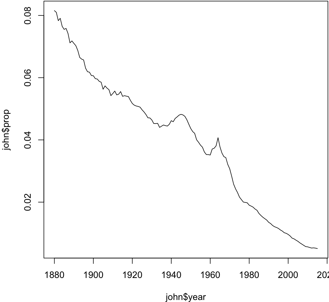

> # Analyzing the name 'Bella'
> bella <- babynames %>% filter(sex=="F", name=="Bella") 
> plot(bella$year, bella$prop, type="l")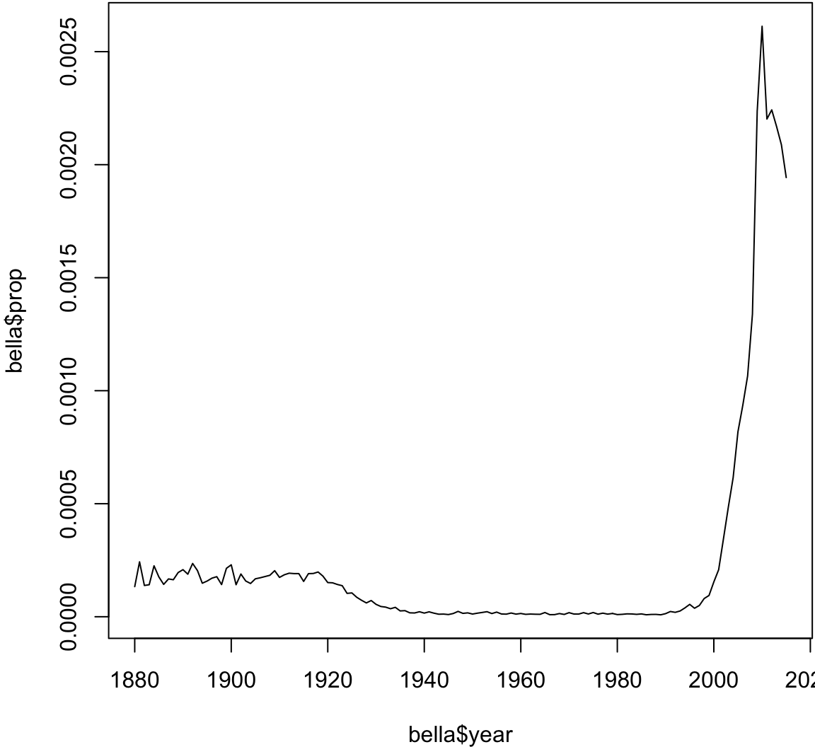

Additional Examples

You should study additional tutorials of dplyr that utilize other data sets:

Read the dplyr introductory vignette
Read the examples given in the R for Data Science assigned reading

Additional `dplyr` Features

We’ve only scratched the surface – many interesting demos of dplyr can be found online
dplyr can work with other data frame backends such as SQL databases
There is an SQL interface for relational databases via the DBI package
dplyr can be integrated with the data.table package for large fast tables
There is a healthy rivalry between dplyr and data.table

Relational Data

Multiple Data Sets

In many data analyses you will have multiple tables of related data that must be combined in order to carry out your analysis.

The dplyr package includes a number of tools to facilitate this.

Toy Example

Here are two data frames that are related through a common variable called key.

> x <- tibble(key = c(1, 2, 3), x_val = c("x1", "x2", "x3"))
> y <- tibble(key = c(1, 2, 4), y_val = c("y1", "y2", "y4"))

> x
# A tibble: 3 × 2
    key x_val
  <dbl> <chr>
1     1    x1
2     2    x2
3     3    x3
> y
# A tibble: 3 × 2
    key y_val
  <dbl> <chr>
1     1    y1
2     2    y2
3     4    y4

Verbs

To work with relational data you need verbs that work with pairs of tables. There are three families of verbs designed to work with relational data.

Mutating joins add new variables to one data frame from matching observations in another.
Filtering joins filter observations from one data frame based on whether or not they match an observation in the other table.
Set operations treat observations as if they were set elements.

From R for Data Science

`inner_join()`

An inner-join matches pairs of observations when their keys are equal.

> inner_join(x, y, key="key")
Joining, by = "key"
# A tibble: 2 × 3
    key x_val y_val
  <dbl> <chr> <chr>
1     1    x1    y1
2     2    x2    y2

`left_join()`

A left-join keeps all observations in the first argument, x.

> left_join(x, y, key="key")
Joining, by = "key"
# A tibble: 3 × 3
    key x_val y_val
  <dbl> <chr> <chr>
1     1    x1    y1
2     2    x2    y2
3     3    x3  <NA>

> x %>% left_join(y, key="key")
Joining, by = "key"
# A tibble: 3 × 3
    key x_val y_val
  <dbl> <chr> <chr>
1     1    x1    y1
2     2    x2    y2
3     3    x3  <NA>

`right_join()`

A right-join keeps all observations in the second argument, y.

> right_join(x, y)
Joining, by = "key"
# A tibble: 3 × 3
    key x_val y_val
  <dbl> <chr> <chr>
1     1    x1    y1
2     2    x2    y2
3     4  <NA>    y4

`full_join()`

A full-join keeps all observations in either argument, x or y.

> full_join(x, y, key="key")
Joining, by = "key"
# A tibble: 4 × 3
    key x_val y_val
  <dbl> <chr> <chr>
1     1    x1    y1
2     2    x2    y2
3     3    x3  <NA>
4     4  <NA>    y4

`anti_join()`

An anti-join removes all observations in the first argument, x, that appear in the second argument, y.

> anti_join(x, y, key="key")
Joining, by = "key"
# A tibble: 1 × 2
    key x_val
  <dbl> <chr>
1     3    x3

`semi_join()`

A semi-join keeps all observations in the first argument, x, that have a match in the second argument, y.

> semi_join(x, y, key="key")
Joining, by = "key"
# A tibble: 2 × 2
    key x_val
  <dbl> <chr>
1     1    x1
2     2    x2

Repeated Key Values

When one of the two data frames has repeated key values, the observations are repeated in the other data frame.

> y2
# A tibble: 4 × 2
    key y_val
  <dbl> <chr>
1     1    y1
2     2   y2a
3     2   y2b
4     4    y4

> x %>% left_join(y2, key="key")
Joining, by = "key"
# A tibble: 4 × 3
    key x_val y_val
  <dbl> <chr> <chr>
1     1    x1    y1
2     2    x2   y2a
3     2    x2   y2b
4     3    x3  <NA>

Set Operations

One can perform traditional set operations on the rows of data frames.

intersect(x, y): return only observations in both x and y
union(x, y): return unique observations in x and y
setdiff(x, y): return observations in x, but not in y

From R for Data Science

Example `setdiff()`

> df1
# A tibble: 2 × 2
      x     y
  <dbl> <dbl>
1     1     1
2     2     1
> df2
# A tibble: 2 × 2
      x     y
  <dbl> <dbl>
1     1     1
2     1     2
> setdiff(df1, df2)
# A tibble: 1 × 2
      x     y
  <dbl> <dbl>
1     2     1

Getting Data In and Out of R

`.RData` Files

R objects can be saved to binary .RData files and loaded with the save (or save.image) and load functions, respectively.

This is the easiest way to get data into R.

`readr` Package

There are a number of R packages that provide more sophisticated tools for getting data in and out of R, especially as data sets have become larger and larger.

One of those packages is readr for text files. It reads and writes data quickly, provides a useful status bar for large files, and does a good job at determining data types.

readr is organized similarly to the base R functions. For example, there are functions read_table, read_csv, write_tsv, and write_csv.

See also fread and fwrite from the data.table package.

Scraping from the Web (Ex. 1)

There are several packages that facilitate “scraping” data from the web, including rvest demonstrated here.

> library("rvest")
> schedule <- read_html("http://jdstorey.github.io/asdscourse/schedule/")
> first_table <- html_table(schedule)[[1]]
> names(first_table) <- c("week", "topics", "reading")
> first_table[2,"week"]
[1] 2
> first_table[2,"topics"] %>% strsplit(split="  ")
[[1]]
[1] "Data Wrangling"
> first_table[2,"reading"] %>% strsplit(split="  ")
[[1]]
[1] "R4DS Ch. 5, 9-16"
> grep("R4DS", first_table$reading) # which rows (weeks) have R4DS
[1] 1 2 3

Scraping from the Web (Ex. 2)

The rvest documentation recommends SelectorGadget, which is “a javascript bookmarklet that allows you to interactively figure out what css selector you need to extract desired components from a page.”

> usg_url <- "http://princetonusg.com/meet-your-usg-officers/"
> usg <- read_html(usg_url)
> officers <- html_nodes(usg, ".team-member-name") %>% 
+             html_text
> head(officers, n=20)
 [1] "Myesha Jemison"       "Daniel Qian"         
 [3] "Alison Shim"          "Katherine Wang"      
 [5] "Pooja Patel"          "Miranda Rosen"       
 [7] "Michael Asparrin"     "Devin Kilpatrick"    
 [9] "Pritika Mehra"        "Olivia Grah"         
[11] "Lucas Ramos"          "Ellie Shannon"       
[13] "Nicholas Wu"          "Wendy Zhao"          
[15] "Soraya Morales Nuñez" "Eli Schechner"       
[17] "Ruby Guo"             "Andrew Ma"           
[19] "Nate Lambert"         "June Philippe"

APIs

API stands for “application programming interface” which is a set of routines, protocols, and tools for building software and applications.

A specific website may provide an API for scraping data from that website.

There are R packages that provide an interface with specific APIs, such as the twitteR package.

Case Study

Yeast Genomics

Smith and Kruglyak (2008) is a study that measured 2820 genotypes in 109 yeast F1 segregants from a cross between parental lines BY and RM.

They also measured gene expression on 4482 genes in each of these segregants when growing in two different Carbon sources, glucose and ethanol.

Load Data

The data was distributed as a collection of matrices in R.

> rm(list=ls())
> load("./data/smith_kruglyak.RData")
> ls()
[1] "exp.e"      "exp.g"      "exp.pos"    "marker"    
[5] "marker.pos"
> eapply(env=.GlobalEnv, dim)
$exp.e
[1] 4482  109

$exp.g
[1] 4482  109

$marker
[1] 2820  109

$exp.pos
[1] 4482    3

$marker.pos
[1] 2820    2

Gene Expression Matrices

> exp.g %>% cbind(rownames(exp.g), .) %>% as_tibble() %>% 
+   print()
# A tibble: 4,482 × 110
        `` X100g.20_4_c.glucose X101g.21_1_d.glucose
     <chr>                <chr>                <chr>
1  YJR107W                 0.22                 0.18
2  YPL270W                -0.29                 -0.2
3  YDR518W                 0.72                 0.04
4  YDR233C                 0.23                 0.31
5  YHR098C                  0.4                -0.04
6  YFR029W                -0.36                 0.35
7  YPL198W                 0.23                -0.21
8  YDR001C                -0.09                 0.57
9  YLR394W                -0.23                 0.13
10 YCR079W                -0.25                -0.98
# ... with 4,472 more rows, and 107 more variables:
#   X102g.21_2_d.glucose <chr>, X103g.21_3_d.glucose <chr>,
#   X104g.21_4_d.glucose <chr>, X105g.21_5_c.glucose <chr>,
#   X106g.22_2_d.glucose <chr>, X107g.22_3_b.glucose <chr>,
#   X109g.22_5_d.glucose <chr>, X10g.2_5_d.glucose <chr>,
#   X110g.23_3_d.glucose <chr>, X111g.23_5_d.glucose <chr>,
#   X112g.24_1_d.glucose <chr>, X113g.25_1_d.glucose <chr>,
#   X114g.25_3_d.glucose <chr>, X115g.25_4_d.glucose <chr>,
#   X116g.26_1_d.glucose <chr>, X117g.26_2_d.glucose <chr>,
#   X11g.2_6_d.glucose <chr>, X12g.2_7_a.glucose <chr>,
#   X13g.3_1_d.glucose <chr>, X15g.3_3_d.glucose <chr>,
#   X16g.3_4_d.glucose <chr>, X17g.3_5_d.glucose <chr>,
#   X18g.4_1_c.glucose <chr>, X1g.1_1_d.glucose <chr>,
#   X20g.4_3_d.glucose <chr>, X21g.4_4_d.glucose <chr>,
#   X22g.5_1_d.glucose <chr>, X23g.5_2_d.glucose <chr>,
#   X24g.5_3_d.glucose <chr>, X25g.5_4_d.glucose <chr>,
#   X26g.5_5_d.glucose <chr>, X27g.6_1_d.glucose <chr>,
#   X28g.6_2_b.glucose <chr>, X29g.6_3_c.glucose <chr>,
#   X30g.6_4_d.glucose <chr>, X31g.6_5_d.glucose <chr>,
#   X32g.6_6_d.glucose <chr>, X33g.6_7_d.glucose <chr>,
#   X34g.7_1_d.glucose <chr>, X35g.7_2_c.glucose <chr>,
#   X36g.7_3_d.glucose <chr>, X37g.7_4_c.glucose <chr>,
#   X38g.7_5_d.glucose <chr>, X39g.7_6_c.glucose <chr>,
#   X3g.1_3_d.glucose <chr>, X40g.7_7_c.glucose <chr>,
#   X41g.7_8_d.glucose <chr>, X42g.8_1_a.glucose <chr>,
#   X43g.8_2_d.glucose <chr>, X44g.8_3_a.glucose <chr>,
#   X45g.8_4_c.glucose <chr>, X46g.8_5_b.glucose <chr>,
#   X47g.8_6_c.glucose <chr>, X48g.8_7_b.glucose <chr>,
#   X49g.9_1_d.glucose <chr>, X4g.1_4_d.glucose <chr>,
#   X50g.9_2_d.glucose <chr>, X51g.9_3_d.glucose <chr>,
#   X52g.9_4_d.glucose <chr>, X53g.9_5_d.glucose <chr>,
#   X54g.9_6_d.glucose <chr>, X55g.9_7_d.glucose <chr>,
#   X56g.10_1_c.glucose <chr>, X57g.10_2_d.glucose <chr>,
#   X58g.10_3_c.glucose <chr>, X59g.10_4_d.glucose <chr>,
#   X5g.1_5_c.glucose <chr>, X60g.11_1_a.glucose <chr>,
#   X61g.11_2_d.glucose <chr>, X62g.11_3_b.glucose <chr>,
#   X63g.12_1_d.glucose <chr>, X64g.12_2_b.glucose <chr>,
#   X65g.13_1_a.glucose <chr>, X66g.13_2_c.glucose <chr>,
#   X67g.13_3_b.glucose <chr>, X68g.13_4_a.glucose <chr>,
#   X69g.13_5_c.glucose <chr>, X70g.14_1_b.glucose <chr>,
#   X71g.14_2_c.glucose <chr>, X73g.14_4_a.glucose <chr>,
#   X74g.14_5_b.glucose <chr>, X75g.14_6_d.glucose <chr>,
#   X76g.14_7_c.glucose <chr>, X77g.15_2_d.glucose <chr>,
#   X78g.15_3_b.glucose <chr>, X79g.15_4_d.glucose <chr>,
#   X7g.2_2_d.glucose <chr>, X80g.15_5_b.glucose <chr>,
#   X82g.16_1_d.glucose <chr>, X83g.17_1_a.glucose <chr>,
#   X84g.17_2_d.glucose <chr>, X85g.17_4_a.glucose <chr>,
#   X86g.17_5_b.glucose <chr>, X87g.18_1_d.glucose <chr>,
#   X88g.18_2_d.glucose <chr>, X89g.18_3_d.glucose <chr>,
#   X8g.2_3_d.glucose <chr>, X90g.18_4_c.glucose <chr>,
#   X92g.19_1_c.glucose <chr>, X93g.19_2_c.glucose <chr>, ...

Gene Position Matrix

> exp.pos %>% cbind(rownames(exp.pos), .) %>% as_tibble() %>% 
+   print()
# A tibble: 4,482 × 4
        `` Chromsome Start_coord End_coord
     <chr>     <chr>       <chr>     <chr>
1  YJR107W        10      627333    628319
2  YPL270W        16       30482     32803
3  YDR518W         4     1478600   1480153
4  YDR233C         4      930353    929466
5  YHR098C         8      301937    299148
6  YFR029W         6      210925    212961
7  YPL198W        16      173151    174701
8  YDR001C         4      452472    450217
9  YLR394W        12      907950    909398
10 YCR079W         3      252842    254170
# ... with 4,472 more rows

Row Names

The gene names are contained in the row names.

> head(rownames(exp.g))
[1] "YJR107W" "YPL270W" "YDR518W" "YDR233C" "YHR098C" "YFR029W"
> head(rownames(exp.e))
[1] "YJR107W" "YPL270W" "YDR518W" "YDR233C" "YHR098C" "YFR029W"
> head(rownames(exp.pos))
[1] "YJR107W" "YPL270W" "YDR518W" "YDR233C" "YHR098C" "YFR029W"
> all.equal(rownames(exp.g), rownames(exp.e))
[1] TRUE
> all.equal(rownames(exp.g), rownames(exp.pos))
[1] TRUE

Unify Column Names

The segregants are column names, and they are inconsistent across matrices.

> head(colnames(exp.g))
[1] "X100g.20_4_c.glucose" "X101g.21_1_d.glucose"
[3] "X102g.21_2_d.glucose" "X103g.21_3_d.glucose"
[5] "X104g.21_4_d.glucose" "X105g.21_5_c.glucose"
> head(colnames(marker))
[1] "20_4_c" "21_1_d" "21_2_d" "21_3_d" "21_4_d" "21_5_c"
>      
> #fix column names with gsub
> colnames(exp.g) %<>% strsplit(split=".", fixed=TRUE) %>%
+   lapply(function(x) {x[2]})
> colnames(exp.e) %<>% strsplit(split=".", fixed=TRUE) %>%
+   lapply(function(x) {x[2]})
> head(colnames(exp.g))
[1] "20_4_c" "21_1_d" "21_2_d" "21_3_d" "21_4_d" "21_5_c"

Gene Positions

Let’s first pull out rownames of exp.pos and make them a column in the data frame.

> gene_pos <- exp.pos %>% as_tibble() %>%
+   mutate(gene = rownames(exp.pos)) %>%
+   dplyr::select(gene, chr = Chromsome, start = Start_coord, 
+                 end = End_coord)
> print(gene_pos, n=7)
# A tibble: 4,482 × 4
     gene   chr   start     end
    <chr> <int>   <int>   <int>
1 YJR107W    10  627333  628319
2 YPL270W    16   30482   32803
3 YDR518W     4 1478600 1480153
4 YDR233C     4  930353  929466
5 YHR098C     8  301937  299148
6 YFR029W     6  210925  212961
7 YPL198W    16  173151  174701
# ... with 4,475 more rows

Tidy Each Expression Matrix

We melt the expression matrices and bind them together into one big tidy data frame.

> exp_g <- melt(exp.g) %>% as_tibble() %>% 
+   dplyr::select(gene = Var1, segregant = Var2, 
+                 expression = value) %>%
+   mutate(condition = "glucose")
> exp_e <- melt(exp.e) %>% as_tibble() %>% 
+   dplyr::select(gene = Var1, segregant = Var2, 
+                 expression = value) %>%
+   mutate(condition = "ethanol")
> print(exp_e, n=4)
# A tibble: 488,538 × 4
     gene segregant expression condition
   <fctr>    <fctr>      <dbl>     <chr>
1 YJR107W    20_4_c       0.06   ethanol
2 YPL270W    20_4_c      -0.13   ethanol
3 YDR518W    20_4_c      -0.94   ethanol
4 YDR233C    20_4_c       0.04   ethanol
# ... with 4.885e+05 more rows

Combine Into Single Data Frame

Combine gene expression data from two conditions into a single data frame.

> exp_all <- bind_rows(exp_g, exp_e)
> sample_n(exp_all, size=10)
# A tibble: 10 × 4
      gene segregant expression condition
    <fctr>    <fctr>      <dbl>     <chr>
1  YBL087C    21_4_d      -0.72   ethanol
2  YDR524C    21_2_d      -0.17   glucose
3  YGR067C     9_1_d      -3.92   glucose
4  YHR207C    26_1_d      -0.43   ethanol
5  YDR329C    20_2_d      -0.06   glucose
6  YGL121C     8_7_b       1.00   ethanol
7  YJR044C     3_3_d      -0.12   ethanol
8  YIL088C     2_7_a       0.10   ethanol
9  YML127W     5_1_d      -0.08   ethanol
10 YMR304W     6_1_d       0.20   ethanol

Join Gene Positions

Now we want to join the gene positions with the expression data.

> exp_all <- exp_all %>%
+   mutate(gene = as.character(gene), 
+          segregant = as.character(segregant))
> sk_tidy <- exp_all %>%
+   left_join(gene_pos, by = "gene")
> sample_n(sk_tidy, size=7)
# A tibble: 7 × 7
     gene segregant expression condition   chr  start    end
    <chr>     <chr>      <dbl>     <chr> <int>  <int>  <int>
1 YGL189C     1_3_d      -0.26   ethanol     7 148594 148235
2 YBR257W    13_2_c       0.02   ethanol     2 728880 729719
3 YER098W    21_1_d       0.46   ethanol     5 355462 357726
4 YCR035C     9_1_d       0.07   glucose     3 193014 191830
5 YBR097W    17_5_b      -0.03   glucose     2 436945 441309
6 YBR235W     8_4_c      -0.18   ethanol     2 686896 690258
7 YJL094C    14_6_d       0.00   glucose    10 254437 251816

Apply `dplyr` Functions

Now that we have the data made tidy in the data frame sk_tidy, let’s apply some dplyr operations…

Does each gene have the same number of observations?

> sk_tidy %>% group_by(gene) %>% 
+   summarize(value = n()) %>%
+   summary()
     gene               value      
 Length:4478        Min.   :218.0  
 Class :character   1st Qu.:218.0  
 Mode  :character   Median :218.0  
                    Mean   :218.6  
                    3rd Qu.:218.0  
                    Max.   :872.0

No, so let’s see which genes have more than one set of observations.

> sk_tidy %>% group_by(gene) %>% 
+   summarize(value = n()) %>%
+   filter(value > median(value))
# A tibble: 4 × 2
       gene value
      <chr> <int>
1 YFR024C-A   872
2   YJL012C   872
3   YKL198C   872
4   YPR089W   872

Let’s remove replicated measurements for these genes.

> sk_tidy %<>% distinct(gene, segregant, condition, 
+                       .keep_all = TRUE)
> 
> sk_tidy %>% group_by(gene) %>% 
+   summarize(value = n()) %>%
+   summary()
     gene               value    
 Length:4478        Min.   :218  
 Class :character   1st Qu.:218  
 Mode  :character   Median :218  
                    Mean   :218  
                    3rd Qu.:218  
                    Max.   :218

As an exercise, think about how you would use dplyr to replace the replicated gene expression values with a single averaged expression value for these genes.

Get the mean and standard deviation expression per chromosome.

> sk_tidy %>%
+   group_by(chr) %>%
+   summarize(mean = mean(expression), sd=sd(expression))
# A tibble: 16 × 3
     chr        mean        sd
   <int>       <dbl>     <dbl>
1      1 -0.07618458 0.8257397
2      2 -0.04471450 0.6322533
3      3 -0.02296456 0.6815490
4      4 -0.02325893 0.5368523
5      5 -0.05793524 0.6098741
6      6 -0.07721815 0.6598159
7      7 -0.04409662 0.6174735
8      8 -0.04743984 0.6377910
9      9 -0.04298423 0.6144313
10    10 -0.02994634 0.5701558
11    11 -0.03964107 0.6130319
12    12 -0.05146305 0.6432055
13    13 -0.02646819 0.5835865
14    14 -0.02943206 0.6423964
15    15 -0.01301063 0.5544749
16    16 -0.03681626 0.6044444

Get the mean and standard deviation expression per chromosome in each condition.

> sk_tidy %>%
+   group_by(chr, condition) %>%
+   summarize(mean = mean(expression), sd=sd(expression))
Source: local data frame [32 x 4]
Groups: chr [?]

     chr condition          mean        sd
   <int>     <chr>         <dbl>     <dbl>
1      1   ethanol  0.0260098709 0.4796494
2      1   glucose -0.1783790350 1.0549134
3      2   ethanol  0.0131661446 0.4793614
4      2   glucose -0.1025951501 0.7503419
5      3   ethanol  0.0001644526 0.5360078
6      3   glucose -0.0460935780 0.8004235
7      4   ethanol  0.0018726571 0.4817756
8      4   glucose -0.0483905104 0.5857082
9      5   ethanol -0.0297045435 0.4787130
10     5   glucose -0.0861659403 0.7163443
# ... with 22 more rows

Count the number of genes per chromosome.

> sk_tidy %>%
+   filter(condition == "glucose", segregant == "20_4_c") %>%
+   group_by(chr) %>% 
+   summarize(num.genes = n())
# A tibble: 16 × 2
     chr num.genes
   <int>     <int>
1      1        60
2      2       298
3      3       125
4      4       629
5      5       207
6      6        79
7      7       395
8      8       209
9      9       152
10    10       256
11    11       241
12    12       387
13    13       367
14    14       319
15    15       388
16    16       366

Filter for the first gene on every chromosome.

> sk_tidy %>%
+   filter(condition == "glucose", segregant == "20_4_c") %>%
+   group_by(chr) %>%
+   filter(start == min(start))
Source: local data frame [16 x 7]
Groups: chr [16]

      gene segregant expression condition   chr start   end
     <chr>     <chr>      <dbl>     <chr> <int> <int> <int>
1  YHL040C    20_4_c      -2.79   glucose     8 20968 19085
2  YNL334C    20_4_c      -0.90   glucose    14 12876 12208
3  YOL157C    20_4_c      -1.06   glucose    15 24293 22524
4  YKL222C    20_4_c       0.09   glucose    11  5621  3504
5  YIL168W    20_4_c      -1.14   glucose     9 29032 29415
6  YJL213W    20_4_c       0.84   glucose    10 32163 33158
7  YPL272C    20_4_c      -0.18   glucose    16 28164 26611
8  YLL063C    20_4_c      -0.66   glucose    12 16072 14648
9  YFL048C    20_4_c      -0.09   glucose     6 40180 38843
10 YML132W    20_4_c      -0.21   glucose    13  7244  8383
11 YGL261C    20_4_c      -0.14   glucose     7  6652  6290
12 YBL107C    20_4_c       0.29   glucose     2 10551  9961
13 YDL248W    20_4_c      -0.68   glucose     4  1802  2953
14 YEL073C    20_4_c      -0.02   glucose     5  7553  7230
15 YAL062W    20_4_c      -5.64   glucose     1 31568 32941
16 YCL068C    20_4_c       0.47   glucose     3 12285 11503

To plot expression in glucose versus ethanol we first need to use dcast().

> sk_tidy %>% dcast(gene + segregant ~ condition, 
+                   value.var = "expression") %>%
+   as_tibble()
# A tibble: 488,102 × 4
      gene segregant ethanol glucose
     <chr>     <chr>   <dbl>   <dbl>
1  YAL002W     1_1_d    0.37   -0.01
2  YAL002W     1_3_d    0.23    0.03
3  YAL002W     1_4_d    0.08    0.07
4  YAL002W     1_5_c   -0.12    0.13
5  YAL002W    10_1_c    0.12   -0.10
6  YAL002W    10_2_d    0.10   -0.20
7  YAL002W    10_3_c    0.07   -0.15
8  YAL002W    10_4_d    0.06   -0.04
9  YAL002W    11_1_a    0.07   -0.07
10 YAL002W    11_2_d    0.30    0.10
# ... with 488,092 more rows

> sk_tidy %>% dcast(gene + segregant ~ condition, 
+                   value.var = "expression") %>%
+   filter(gene == "YAL002W") %>%
+   ggplot(aes(x = glucose, y = ethanol)) +
+   geom_point() +  theme_bw() +
+   theme(legend.position = "none")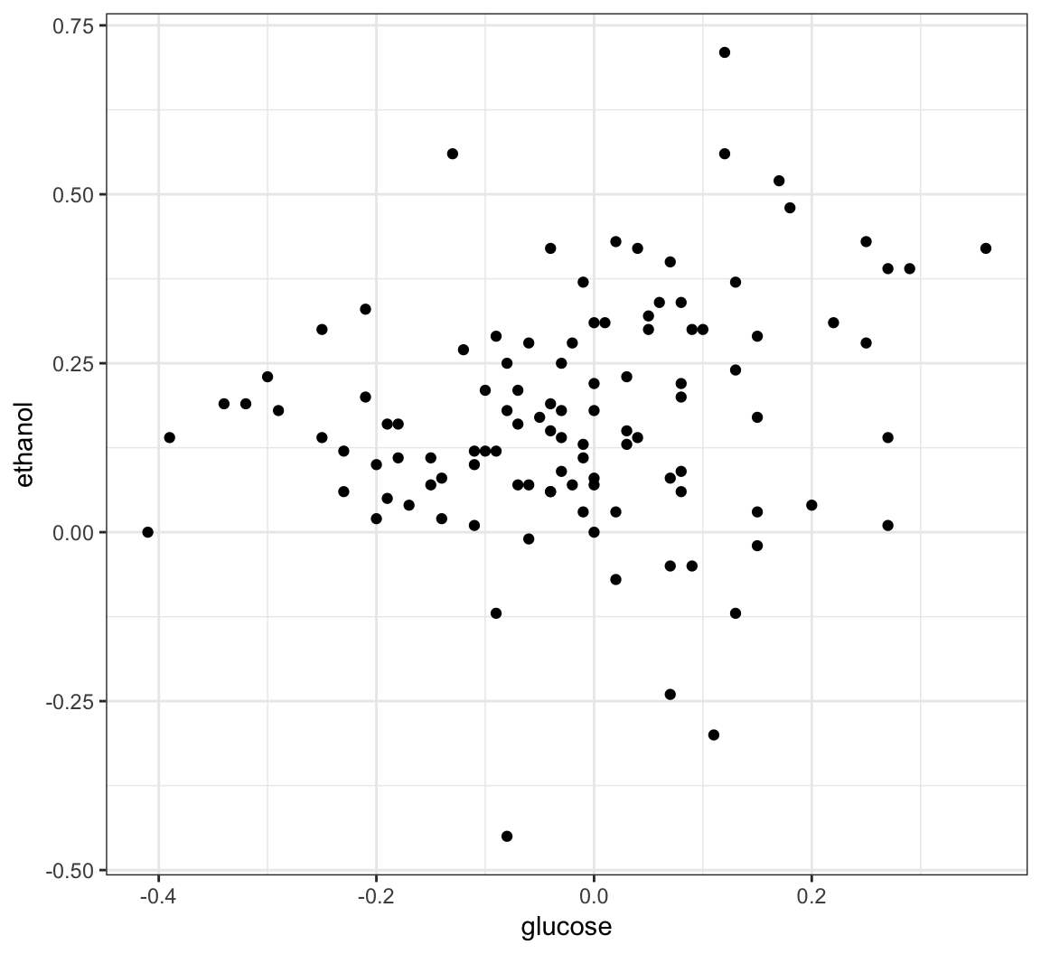

Extras

Source

License

Source Code

Session Information

> sessionInfo()
R version 3.3.2 (2016-10-31)
Platform: x86_64-apple-darwin13.4.0 (64-bit)
Running under: macOS Sierra 10.12.4

locale:
[1] en_US.UTF-8/en_US.UTF-8/en_US.UTF-8/C/en_US.UTF-8/en_US.UTF-8

attached base packages:
[1] stats     graphics  grDevices utils     datasets  methods  
[7] base     

other attached packages:
 [1] rvest_0.3.2     xml2_1.1.1      babynames_0.3.0
 [4] reshape2_1.4.2  dplyr_0.5.0     purrr_0.2.2    
 [7] readr_1.1.0     tidyr_0.6.2     tibble_1.3.0   
[10] ggplot2_2.2.1   tidyverse_1.1.1 knitr_1.15.1   
[13] magrittr_1.5    devtools_1.12.0

loaded via a namespace (and not attached):
 [1] Rcpp_0.12.10     cellranger_1.1.0 plyr_1.8.4      
 [4] forcats_0.2.0    tools_3.3.2      digest_0.6.12   
 [7] lubridate_1.6.0  jsonlite_1.4     evaluate_0.10   
[10] memoise_1.1.0    nlme_3.1-131     gtable_0.2.0    
[13] lattice_0.20-35  psych_1.7.5      DBI_0.6-1       
[16] curl_2.6         yaml_2.1.14      parallel_3.3.2  
[19] haven_1.0.0      withr_1.0.2      stringr_1.2.0   
[22] httr_1.2.1       revealjs_0.9     hms_0.3         
[25] rprojroot_1.2    grid_3.3.2       R6_2.2.0        
[28] XML_3.98-1.7     readxl_1.0.0     foreign_0.8-68  
[31] rmarkdown_1.5    selectr_0.3-1    modelr_0.1.0    
[34] backports_1.0.5  scales_0.4.1     htmltools_0.3.6 
[37] assertthat_0.2.0 mnormt_1.5-5     colorspace_1.3-2
[40] labeling_0.3     stringi_1.1.5    lazyeval_0.2.0  
[43] munsell_0.4.3    broom_0.4.2

QCB 508 – Week 2

John D. Storey

Spring 2017

Data Wrangling

Definition

Workflow

Challenges

Tidy Data

Motivation

Definition

Example: Titanic Data

Intuitive Format

Tidy Format

Rules of Thumb

Tidyverse

Idea

Packages

Primary Packages

Loading tidyverse

Tidying Data

tidyr Package

Untidy Titanic Data

gather()

spread()

Tidy with spread()

Reshaping Data

Wide vs. Long Format

reshape2 Package

Air Quality Data Set

Melt

Guided Melt

Casting

dcast()

Transforming Data

dplyr Package

Grammar of dplyr

Example: Baby Names

babynames Object

Peek at the Data

%>% Operator

filter()

arrange()

arrange()

rename()

select()

Renaming with select()

mutate()

No. Individuals by Year and Sex

summarize()

group_by()

No. Individuals by Year and Sex

How Many Distinct Names?

Most Popular Names

Most Popular Names

Recent Years

Most Popular Female Names

1990s

Most Popular Male Names

1990s

Additional Examples

Additional dplyr Features

Relational Data

Multiple Data Sets

Toy Example

Verbs

inner_join()

left_join()

right_join()

full_join()

anti_join()

semi_join()

Repeated Key Values

Set Operations

Example setdiff()

Getting Data In and Out of R

.RData Files

readr Package

Scraping from the Web (Ex. 1)

Scraping from the Web (Ex. 2)

APIs

Loading `tidyverse`

`tidyr` Package

`gather()`

`spread()`

Tidy with `spread()`

`reshape2` Package

`dcast()`

`dplyr` Package

Grammar of `dplyr`

`babynames` Object

`%>%` Operator

`filter()`

`arrange()`

`arrange()`

`rename()`

`select()`

Renaming with `select()`

`mutate()`

`summarize()`

`group_by()`

Additional `dplyr` Features

`inner_join()`

`left_join()`

`right_join()`

`full_join()`

`anti_join()`

`semi_join()`

Example `setdiff()`

`.RData` Files

`readr` Package

Apply `dplyr` Functions