QCB 508 – Week 1
John D. Storey
Spring 2017
Statistics and Data Science
Statistics
Statistics is the study of the collection, analysis, interpretation, presentation, and organization of data.
Applied Statistics
Applied Statistics is concerned with the practical considerations and implementations needed to carry out a statistical analysis.
Machine Learning
Machine learning explores the study and construction of algorithms that can learn from and make predictions on data. Machine learning is closely related to and often overlaps with computational statistics; a discipline which also focuses in prediction-making through the use of computers.
Data Science
Data Science is an interdisciplinary field about processes and systems to extract knowledge or insights from data in various forms, either structured or unstructured, which is a continuation of some of the data analysis fields such as statistics, data mining, and predictive analytics.
What is Data Science?
Data Science is a very new term
No well-accepted definition
Statistics, machine learning, and data science are all essentially about extracting knowledge or value from data
DS deals with data in the following ways: collecting, storing, managing, wrangling, exploration, learning, discovery, communication, products
Some History
John Tukey
John Tukey pioneered a field called “exploratory data analysis” (EDA)
From The Future of Data Analysis (1962) Annals of Mathematical Statistics …
For a long time I have thought I was a statistician, interested in inferences from the particular to the general. But as I have watched mathematical statistics evolve, I have had cause to wonder and to doubt.
All in all, I have come to feel that my central interest is in data analysis, which I take to include, among other things: procedures for analyzing data, techniques for interpreting the results of such procedures, ways of planning the gathering of data to make its analysis easier, more precise or more accurate, and all the machinery and results of (mathematical) statistics which apply to analyzing data.
Data analysis is a larger and more varied field than inference, or incisive procedures, or allocation.
IMO, Tukey saw the need for and initiated data science in 1962
David Donoho seems to agree
Jeff Wu
In November 1997, C.F. Jeff Wu gave the inaugural lecture entitled “Statistics = Data Science?”. In this lecture, he characterized statistical work as a trilogy of data collection, data modeling and analysis, and decision making. In his conclusion, he initiated the modern, non-computer science, usage of the term “data science” and advocated that statistics be renamed data science and statisticians data scientists.
William Cleveland
In 2001, William Cleveland introduced data science as an independent discipline, extending the field of statistics to incorporate “advances in computing with data” in his article Data Science: An Action Plan for Expanding the Technical Areas of the Field of Statistics in International Statistical Review
Cleveland establishes six technical areas which he believed to encompass the field of data science
(The above is modified text from Wikipedia.)
Statistics \(\rightarrow\) Data Science
Cleveland’s six area to extend statistics to data science:
- multidisciplinary investigations
- models and methods for data
- computing with data
- pedagogy
- tool evaluation
- theory
Industry
“In 2008, DJ Patil and Jeff Hammerbacher used the term ‘data scientist’ to define their jobs at LinkedIn and Facebook, respectively.” (from Wikipedia)
The term “data scientist” is now often used to describe positions in industry that primarily involve data, whether it is statistics, machine learning, data curation, or other data-centric activities
Relevant Quotations
Nate Silver
“I think data scientist is a sexed-up term for a statistician.”
http://simplystatistics.org/2013/08/08/data-scientist-is-just-a-sexed-up-word-for-statistician/
“Data science is statistics on a Mac.”
“A data scientist is a statistician who lives in San Francisco.”
“A data scientist is someone who is better at statistics than any software engineer and better at software engineering than any statistician.”
http://datascopeanalytics.com/blog/what-is-a-data-scientist/
Hadley Wickham
“Recently, there has been much hand-wringing about the role of statistics in data science.
I think there are three main steps in a data science project: you collect data (and questions), analyze it (using visualization and models), then communicate the results."
http://bulletin.imstat.org/2014/09/data-science-how-is-it-different-to-statistics%E2%80%89/
“Statistics is a part of data science, not the whole thing. Statistics research focuses on data collection and modelling, and there is little work on developing good questions, thinking about the shape of data, communicating results or building data products.”
http://bulletin.imstat.org/2014/09/data-science-how-is-it-different-to-statistics%E2%80%89/
Jeff Leek
“The key word in Data Science is not Data, it is Science.”
http://simplystatistics.org/2013/12/12/the-key-word-in-data-science-is-not-data-it-is-science/
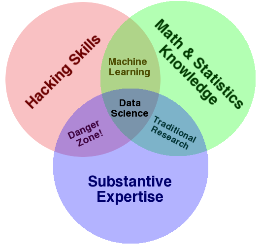
http://drewconway.com/zia/2013/3/26/the-data-science-venn-diagram
QCB 508
What we cover
This course is organized into three parts:
- Wrangling and exploring data
- Statistical inference
- Statistical modeling
What we don’t cover
- Python
- Databases
- Big data computing (e.g., Hadoop, MapReduce, Spark)
- Prediction models
- Deploying data products
Course Logistics
This course will be managed on:
All course notes will be made available on the course web site and GitHub:
The slides will may be organized into a book:
Computing
What is R?
- R is a programming language, a high-level “interpreted language”
- R is an interactive environment
- R is used for doing statistics and data science
Pros and Cons of R
- R is free and open-source
- R stays on the cutting-edge because of its ability to utilize independently developed “packages”
- R has some peculiar featues that experienced programmers should note (see The R Inferno)
- R has an amazing community of passionate users and developers
RStudio
RStudio is an IDE (integrated development environment) for R
It contains many useful features for using R
We will use the free version of RStudio in this course
Getting Started in R
Calculator
Operations on numbers: + - * / ^
> 2+1
[1] 3
> 6+3*4-2^3
[1] 10> 6+(3*4)-(2^3)
[1] 10Atomic Classes
There are five atomic classes (or modes) of objects in R:
- character
- complex
- integer
- logical
- numeric (real number)
There is a sixth called “raw” that we will not discuss.
Assigning Values to Variables
> x <- "qcb508" # character
> x <- 2+1i     # complex
> x <- 4L       # integer
> x <- TRUE     # logical
> x <- 3.14159  # numeric
Note: Anything typed after the # sign is not evaluated. The # sign allows you to add comments to your code.
More Ways to Assign Values
> x <- 1
> 1 -> x
> x = 1
In this class, we ask that you only use x <- 1.
Evaluation
When a complete expression is entered at the prompt, it is evaluated and the result of the evaluated expression is returned. The result may be auto-printed.
> x <- 1
> x+2
[1] 3
> print(x)
[1] 1
> print(x+2)
[1] 3
Functions
There are many useful functions included in R. “Packages” (covered later) can be loaded as libraries to provide additional functions. You can also write your own functions in any R session.
Here are some examples of built-in functions:
> x <- 2
> print(x)
[1] 2
> sqrt(x)
[1] 1.414214
> log(x)
[1] 0.6931472
> class(x)
[1] "numeric"
> is.vector(x)
[1] TRUE
Accessing Help in R
You can open the help file for any function by typing ? with the functions name. Here is an example:
> ?sqrtThere’s also a function help.search that can do general searches for help. You can learn about it by typing:
> ?help.searchIt’s also useful to use Google: for example, “r help square root”. The R help files are also on the web.
Variable Names
In the previous examples, we used x as our variable name. Do not use the following variable names, as they have special meanings in R:
c, q, s, t, C, D, F, I, TWhen combining two words for a given variable, we recommend one of these options:
> my_variable <- 1
> myVariable <- 1
Variable names such as my.variable are problematic because of the special use of “.” in R.
Vectors
The vector is the most basic object in R. You can create vectors in a number of ways.
> x <- c(1, 2, 3, 4, 5)
> x
[1] 1 2 3 4 5
>
> y <- 1:40
> y
 [1]  1  2  3  4  5  6  7  8  9 10 11 12 13 14 15 16 17 18 19
[20] 20 21 22 23 24 25 26 27 28 29 30 31 32 33 34 35 36 37 38
[39] 39 40
>
> z <- seq(from=0, to=100, by=10)
> z
 [1]   0  10  20  30  40  50  60  70  80  90 100
> length(z)
[1] 11
Vectors
- Programmers: vectors are indexed starting at
1, not0 - A vector can only contain elements of a single class:
> x <- "a"
> x[0]
character(0)
> x[1]
[1] "a"
>
> y <- 1:3
> z <- c(x, y, TRUE, FALSE)
> z
[1] "a"     "1"     "2"     "3"     "TRUE"  "FALSE"
Matrices
Like vectors, matrices are objects that can contain elements of only one class.
> m <- matrix(1:6, nrow=2, ncol=3)
> m
     [,1] [,2] [,3]
[1,]    1    3    5
[2,]    2    4    6
>
> m <- matrix(1:6, nrow=2, ncol=3, byrow=TRUE)
> m
     [,1] [,2] [,3]
[1,]    1    2    3
[2,]    4    5    6
Factors
In statistics, factors encode categorical data.
> paint <- factor(c("red", "white", "blue", "blue", "red",
+                   "red"))
> paint
[1] red   white blue  blue  red   red
Levels: blue red white
>
> table(paint)
paint
 blue   red white
    2     3     1
> unclass(paint)
[1] 2 3 1 1 2 2
attr(,"levels")
[1] "blue"  "red"   "white"
Lists
Lists allow you to hold different classes of objects in one variable.
> x <- list(1:3, "a", c(TRUE, FALSE))
> x
[[1]]
[1] 1 2 3

[[2]]
[1] "a"

[[3]]
[1]  TRUE FALSE
>
> # access any element of the list
> x[[2]]
[1] "a"
> x[[3]][2]
[1] FALSE
Lists with Names
The elements of a list can be given names.
> x <- list(counting=1:3, char="a", logic=c(TRUE, FALSE))
> x
$counting
[1] 1 2 3

$char
[1] "a"

$logic
[1]  TRUE FALSE
>
> # access any element of the list
> x$char
[1] "a"
> x$logic[2]
[1] FALSE
Missing Values
In data analysis and model fitting, we often have missing values. NA represents missing values and NaN means “not a number”, which is a special type of missing value.
> m <- matrix(nrow=3, ncol=3)
> m
     [,1] [,2] [,3]
[1,]   NA   NA   NA
[2,]   NA   NA   NA
[3,]   NA   NA   NA
> 0/1
[1] 0
> 1/0
[1] Inf
> 0/0
[1] NaN
NULL
NULL is a special type of reserved value in R.
> x <- vector(mode="list", length=3)
> x
[[1]]
NULL

[[2]]
NULL

[[3]]
NULL
Coercion
We saw earlier that when we mixed classes in a vector they were all coerced to be of type character:
> c("a", 1:3, TRUE, FALSE)
[1] "a"     "1"     "2"     "3"     "TRUE"  "FALSE"
You can directly apply coercion with functions as.numeric(), as.character(), as.logical(), etc.
This doesn’t always work out well:
> x <- 1:3
> as.character(x)
[1] "1" "2" "3"
>
> y <- c("a", "b", "c")
> as.numeric(y)
Warning: NAs introduced by coercion
[1] NA NA NA
Data Frames
The data frame is one of the most important objects in R. Data sets very often come in tabular form of mixed classes, and data frames are constructed exactly for this.
Data frames are lists where each element has the same length.
Data Frames
> df <- data.frame(counting=1:3, char=c("a", "b", "c"),
+                  logic=c(TRUE, FALSE, TRUE))
> df
  counting char logic
1        1    a  TRUE
2        2    b FALSE
3        3    c  TRUE
>
> nrow(df)
[1] 3
> ncol(df)
[1] 3
Data Frames
> dim(df)
[1] 3 3
>
> names(df)
[1] "counting" "char"     "logic"
>
> attributes(df)
$names
[1] "counting" "char"     "logic"

$row.names
[1] 1 2 3

$class
[1] "data.frame"
Attributes
Attributes give information (or meta-data) about R objects. The previous slide shows attributes(df), the attributes of the data frame df.
> x <- 1:3
> attributes(x) # no attributes for a standard vector
NULL
>
> m <- matrix(1:6, nrow=2, ncol=3)
> attributes(m)
$dim
[1] 2 3
> paint <- factor(c("red", "white", "blue", "blue", "red",
+ "red"))
> attributes(paint)
$levels
[1] "blue" "red" "white"
$class
[1] "factor"Names
Names can be assigned to columns and rows of vectors, matrices, and data frames. This makes your code easier to write and read.
> names(x) <- c("Princeton", "Rutgers", "Penn")
> x
Princeton   Rutgers      Penn
        1         2         3
>
> colnames(m) <- c("NJ", "NY", "PA")
> rownames(m) <- c("East", "West")
> m
     NJ NY PA
East  1  3  5
West  2  4  6
> colnames(m)
[1] "NJ" "NY" "PA"
Accessing Names
Displaying or assigning names to these three types of objects does not have consistent syntax.
| Object | Column Names | Row Names |
|---|---|---|
| vector | names() |
N/A |
| data frame | names() |
row.names() |
| data frame | colnames() |
rownames() |
| matrix | colnames() |
rownames() |
Going Deeper
Reproducibility
Definition and Motivation
Reproducibility involves being able to recalculate the exact numbers in a data analysis using the code and raw data provided by the analyst.
Reproducibility is often difficult to achieve and has slowed down the discovery of important data analytic errors.
Reproducibility should not be confused with “correctness” of a data analysis. A data analysis can be fully reproducible and recreate all numbers in an analysis and still be misleading or incorrect.
From Elements of Data Analytic Style, by Leek
Reproducible vs. Replicable
Reproducible research is often used these days to indicate the ability to recalculate the exact numbers in a data analysis
Replicable research results often refers to the ability to independently carry out a study (thereby collecting new data) and coming to equivalent conclusions as the original study
These two terms are often confused, so it is important to clearly state the definition
Steps to a Reproducible Analysis
Use a data analysis script – e.g., R Markdown (discussed next section!) or iPython Notebooks
Record versions of software and paramaters – e.g., use
sessionInfo()in R as inhw_1.RmdOrganize your data analysis
Use version control – e.g., GitHub
Set a random number generator seed – e.g., use
set.seed()in RHave someone else run your analysis
Organizing Your Data Analysis
- Data
- raw data
- processed data (sometimes multiple stages for very large data sets)
- Figures
- Exploratory figures
- Final figures
- R code
- Raw or unused scripts
- Data processing scripts
- Analysis scripts
- Text
- README files explaining what all the components are
- Final data analysis products like presentations/writeups
Common Mistakes
- Failing to use a script for your analysis
- Not recording software and package version numbers or other settings used
- Not sharing your data and code
- Using reproducibility as a social weapon
R Markdown
R + Markdown + knitr
R Markdown was developed by the RStudio team to allow one to write reproducible research documents using Markdown and knitr. This is contained in the rmarkdown package, but can easily be carried out in RStudio.
Markdown was originally developed as a very simply text-to-html conversion tool. With Pandoc, Markdown is a very simply text-to-X conversion tool where X can be many different formats: html, LaTeX, PDF, Word, etc.
R Markdown Files
R Markdown documents begin with a metadata section, the YAML header, that can include information on the title, author, and date as well as options for customizing output.
---
title: "QCB 508 -- Homework 1"
author: "Your Name"
date: February 23, 2017
output: pdf_document
---
Many options are available. See http://rmarkdown.rstudio.com for full documentation.
Markdown
Headers:
# Header 1
## Header 2
### Header 3
Emphasis:
*italic* **bold**
_italic_ __bold__
Tables:
First Header  | Second Header
------------- | -------------
Content Cell  | Content Cell
Content Cell  | Content Cell
Unordered list:
- Item 1
- Item 2
    - Item 2a
    - Item 2b
Ordered list:
1. Item 1
2. Item 2
3. Item 3
    - Item 3a
    - Item 3b
Links:
http://example.com

[linked phrase](http://example.com)
Blockquotes:
Florence Nightingale once said:

> For the sick it is important
> to have the best.
Plain code blocks:
```
This text is displayed verbatim with no formatting.
```
Inline Code:
We use the `print()` function to print the contents
of a variable in R.
Additional documentation and examples can be found here and here.
LaTeX
LaTeX is a markup language for technical writing, especially for mathematics. It can be include in R Markdown files.
For example,
$y = a + bx + \epsilon$produces
\(y = a + bx + \epsilon\)
Here is an introduction to LaTeX and here is a primer on LaTeX for R Markdown.
knitr
The knitr R package allows one to execute R code within a document, and to display the code itself and its output (if desired). This is particularly easy to do in the R Markdown setting. For example…
Placing the following text in an R Markdown file
The sum of 2 and 2 is `r 2+2`.produces in the output file
The sum of 2 and 2 is 4.
knitr Chunks
Chunks of R code separated from the text. In R Markdown:
```{r}
x <- 2
x + 1
print(x)
```
Output in file:
> x <- 2
> x + 1
[1] 3
> print(x)
[1] 2
Chunk Option: echo
In R Markdown:
```{r, echo=FALSE}
x <- 2
x + 1
print(x)
```
Output in file:
[1] 3
[1] 2
Chunk Option: results
In R Markdown:
```{r, results="hide"}
x <- 2
x + 1
print(x)
```
Output in file:
> x <- 2
> x + 1
> print(x)
Chunk Option: include
In R Markdown:
```{r, include=FALSE}
x <- 2
x + 1
print(x)
```
Output in file:
(nothing)
Chunk Option: eval
In R Markdown:
```{r, eval=FALSE}
x <- 2
x + 1
print(x)
```
Output in file:
> x <- 2
> x + 1
> print(x)
Chunk Names
Naming your chunks can be useful for identifying them in your file and during the execution, and also to denote dependencies among chunks.
```{r my_first_chunk}
x <- 2
x + 1
print(x)
```
knitr Option: cache
Sometimes you don’t want to run chunks over and over, especially for large calculations. You can “cache” them.
```{r chunk1, cache=TRUE, include=FALSE}
x <- 2
```
```{r chunk2, cache=TRUE, dependson="chunk1"}
y <- 3
z <- x + y
```This creates a directory called cache in your working directory that stores the objects created or modified in these chunks. When chunk1 is modified, it is re-run. Since chunk2 depends on chunk1, it will also be re-run.
knitr Options: figures
You can add chunk options regarding the placement and size of figures. Examples include:
fig.widthfig.heightfig.align
Changing Default Chunk Settings
If you will be using the same options on most chunks, you can set default options for the entire document. Run something like this at the beginning of your document with your desired chunk options.
```{r my_opts, cache=FALSE, echo=FALSE}
library("knitr")
opts_chunk$set(fig.align="center", fig.height=4, fig.width=6)
```
Documentation and Examples
Control Structures
Rationale
Control structures in R allow you to control the flow of execution of a series of R expressions
They allow you to put some logic into your R code, rather than just always executing the same R code every time
Control structures also allow you to respond to inputs or to features of the data and execute different R expressions accordingly
Paraphrased from R Programming for Data Science, by Peng
Common Control Structures
ifandelse: testing a condition and acting on itfor: execute a loop a fixed number of timeswhile: execute a loop while a condition is truerepeat: execute an infinite loop (must break out of it to stop)break: break the execution of a loopnext: skip an interation of a loop
From R Programming for Data Science, by Peng
Some Boolean Logic
R has built-in functions that produce TRUE or FALSE such as is.vector or is.na. You can also do the following:
x == y: does x equal y?x > y: is x greater than y? (also<less than)x >= y: is x greater than or equal to y?x && y: are both x and y true?x || y: is either x or y true?!is.vector(x): this isTRUEif x is not a vector
if
Idea:
if(<condition>) {
        ## do something
}
## Continue with rest of code
Example:
> x <- c(1,2,3)
> if(is.numeric(x)) {
+   x+2
+ }
[1] 3 4 5if-else
Idea:
if(<condition>) {
        ## do something
}
else {
        ## do something else
}
Example:
> x <- c("a", "b", "c")
> if(is.numeric(x)) {
+   print(x+2)
+ } else {
+   class(x)
+ }
[1] "character"
for Loops
Example:
> for(i in 1:10) {
+   print(i)
+ }
[1] 1
[1] 2
[1] 3
[1] 4
[1] 5
[1] 6
[1] 7
[1] 8
[1] 9
[1] 10
Examples:
> x <- c("a", "b", "c", "d")
>
> for(i in 1:4) {
+   print(x[i])
+ }
[1] "a"
[1] "b"
[1] "c"
[1] "d"
>
> for(i in seq_along(x)) {
+   print(x[i])
+ }
[1] "a"
[1] "b"
[1] "c"
[1] "d"
Nested for Loops
Example:
> m <- matrix(1:6, nrow=2, ncol=3, byrow=TRUE)
>
> for(i in seq_len(nrow(m))) {
+   for(j in seq_len(ncol(m))) {
+     print(m[i,j])
+   }
+ }
[1] 1
[1] 2
[1] 3
[1] 4
[1] 5
[1] 6
while
Example:
> x <- 1:10
> idx <- 1
>
> while(x[idx] < 4) {
+   print(x[idx])
+   idx <- idx + 1
+ }
[1] 1
[1] 2
[1] 3
>
> idx
[1] 4
Repeats the loop until while the condition is TRUE.
repeat
Example:
> x <- 1:10
> idx <- 1
>
> repeat {
+   print(x[idx])
+   idx <- idx + 1
+   if(idx >= 4) {
+     break
+   }
+ }
[1] 1
[1] 2
[1] 3
>
> idx
[1] 4
Repeats the loop until break is executed.
break and next
break ends the loop. next skips the rest of the current loop iteration.
Example:
> x <- 1:1000
> for(idx in 1:1000) {
+   # %% calculates division remainder
+   if((x[idx] %% 2) > 0) {
+     next
+   } else if(x[idx] > 10) { # an else-if!!
+     break
+   } else {
+     print(x[idx])
+   }
+ }
[1] 2
[1] 4
[1] 6
[1] 8
[1] 10
Vectorized Operations
Calculations on Vectors
R is usually smart about doing calculations with vectors. Examples:
>
> x <- 1:3
> y <- 4:6
>
> 2*x     # same as c(2*x[1], 2*x[2], 2*x[3])
[1] 2 4 6
> x + 1   # same as c(x[1]+1, x[2]+1, x[3]+1)
[1] 2 3 4
> x + y   # same as c(x[1]+y[1], x[2]+y[2], x[3]+y[3])
[1] 5 7 9
> x*y     # same as c(x[1]*y[1], x[2]*y[2], x[3]*y[3])
[1]  4 10 18
A Caveat
If two vectors are of different lengths, R tries to find a solution for you (and doesn’t always tell you).
> x <- 1:5
> y <- 1:2
> x+y
Warning in x + y: longer object length is not a multiple of
shorter object length
[1] 2 4 4 6 6
What happened here?
Vectorized Matrix Operations
Operations on matrices are also vectorized. Example:
> x <- matrix(1:4, nrow=2, ncol=2, byrow=TRUE)
> y <- matrix(1:4, nrow=2, ncol=2)
>
> x+y
     [,1] [,2]
[1,]    2    5
[2,]    5    8
>
> x*y
     [,1] [,2]
[1,]    1    6
[2,]    6   16
Mixing Vectors and Matrices
What happens when we do calculations involving a vector and a matrix? Example:
> x <- matrix(1:6, nrow=2, ncol=3, byrow=TRUE)
> z <- 1:2
>
> x + z
     [,1] [,2] [,3]
[1,]    2    3    4
[2,]    6    7    8
>
> x * z
     [,1] [,2] [,3]
[1,]    1    2    3
[2,]    8   10   12
Mixing Vectors and Matrices
Another example:
> x <- matrix(1:6, nrow=2, ncol=3, byrow=TRUE)
> z <- 1:3
>
> x + z
     [,1] [,2] [,3]
[1,]    2    5    5
[2,]    6    6    9
>
> x * z
     [,1] [,2] [,3]
[1,]    1    6    6
[2,]    8    5   18
What happened this time?
Vectorized Boolean Logic
We saw && and || applied to pairs of logical values. We can also vectorize these operations.
> a <- c(TRUE, TRUE, FALSE)
> b <- c(FALSE, TRUE, FALSE)
>
> a | b
[1]  TRUE  TRUE FALSE
> a & b
[1] FALSE  TRUE FALSE
Subsetting R Objects
Subsetting Vectors
> x <- 1:8
>
> x[1]           # extract the first element
[1] 1
> x[2]           # extract the second element
[1] 2
>
> x[1:4]         # extract the first 4 elements
[1] 1 2 3 4
>
> x[c(1, 3, 4)]  # extract elements 1, 3, and 4
[1] 1 3 4
> x[-c(1, 3, 4)] # extract all elements EXCEPT 1, 3, and 4
[1] 2 5 6 7 8
Subsetting Vectors
> names(x) <- letters[1:8]
> x
a b c d e f g h
1 2 3 4 5 6 7 8
>
> x[c("a", "b", "f")]
a b f
1 2 6
>
> s <- x > 3
> s
    a     b     c     d     e     f     g     h
FALSE FALSE FALSE  TRUE  TRUE  TRUE  TRUE  TRUE
> x[s]
d e f g h
4 5 6 7 8
Subsettng Matrices
> x <- matrix(1:6, nrow=2, ncol=3, byrow=TRUE)
> x
     [,1] [,2] [,3]
[1,]    1    2    3
[2,]    4    5    6
>
> x[1,2]
[1] 2
> x[1, ]
[1] 1 2 3
> x[ ,2]
[1] 2 5
Subsettng Matrices
> colnames(x) <- c("A", "B", "C")
>
> x[ , c("B", "C")]
     B C
[1,] 2 3
[2,] 5 6
>
> x[c(FALSE, TRUE), c("B", "C")]
B C
5 6
>
> x[2, c("B", "C")]
B C
5 6
Subsettng Matrices
> s <- (x %% 2) == 0
> s
         A     B     C
[1,] FALSE  TRUE FALSE
[2,]  TRUE FALSE  TRUE
>
> x[s]
[1] 4 2 6
>
> x[c(2, 3, 6)]
[1] 4 2 6
Subsetting Lists
> x <- list(my=1:3, favorite=c("a", "b", "c"),
+           course=c(FALSE, TRUE, NA))
>
> x[[1]]
[1] 1 2 3
> x[["my"]]
[1] 1 2 3
> x$my
[1] 1 2 3
> x[[c(3,1)]]
[1] FALSE
> x[[3]][1]
[1] FALSE> x[c(3,1)]
$course
[1] FALSE TRUE NA
$my
[1] 1 2 3Subsetting Data Frames
> x <- data.frame(my=1:3, favorite=c("a", "b", "c"),
+           course=c(FALSE, TRUE, NA))
>
> x[[1]]
[1] 1 2 3
> x[["my"]]
[1] 1 2 3
> x$my
[1] 1 2 3
> x[[c(3,1)]]
[1] FALSE
> x[[3]][1]
[1] FALSE> x[c(3,1)]
course my
1 FALSE 1
2 TRUE 2
3 NA 3Subsetting Data Frames
> x <- data.frame(my=1:3, favorite=c("a", "b", "c"),
+           course=c(FALSE, TRUE, NA))
>
> x[1, ]
  my favorite course
1  1        a  FALSE
> x[ ,3]
[1] FALSE  TRUE    NA
> x[ ,"favorite"]
[1] a b c
Levels: a b c
> x[1:2, ]
my favorite course
1 1 a FALSE
2 2 b TRUE
> x[ ,2:3]
favorite course
1 a FALSE
2 b TRUE
3 c NANote on Data Frames
R often converts character strings to factors unless you specify otherwise.
In the previous slide, we saw it converted the “favorite” column to factors. Let’s fix that…
> x <- data.frame(my=1:3, favorite=c("a", "b", "c"),
+                 course=c(FALSE, TRUE, NA),
+                 stringsAsFactors=FALSE)
>
> x[ ,"favorite"]
[1] "a" "b" "c"
> class(x[ ,"favorite"])
[1] "character"
Missing Values
> data("airquality", package="datasets")
> head(airquality)
  Ozone Solar.R Wind Temp Month Day
1    41     190  7.4   67     5   1
2    36     118  8.0   72     5   2
3    12     149 12.6   74     5   3
4    18     313 11.5   62     5   4
5    NA      NA 14.3   56     5   5
6    28      NA 14.9   66     5   6
> dim(airquality)
[1] 153   6
> which(is.na(airquality$Ozone))
[1] 5 10 25 26 27 32 33 34 35 36 37 39 42 43
[15] 45 46 52 53 54 55 56 57 58 59 60 61 65 72
[29] 75 83 84 102 103 107 115 119 150
> sum(is.na(airquality$Ozone))
[1] 37Subsetting by Matching
> letters
 [1] "a" "b" "c" "d" "e" "f" "g" "h" "i" "j" "k" "l" "m" "n"
[15] "o" "p" "q" "r" "s" "t" "u" "v" "w" "x" "y" "z"
> vowels <- c("a", "e", "i", "o", "u")
>
> letters %in% vowels
 [1]  TRUE FALSE FALSE FALSE  TRUE FALSE FALSE FALSE  TRUE
[10] FALSE FALSE FALSE FALSE FALSE  TRUE FALSE FALSE FALSE
[19] FALSE FALSE  TRUE FALSE FALSE FALSE FALSE FALSE
> which(letters %in% vowels)
[1]  1  5  9 15 21
>
> letters[which(letters %in% vowels)]
[1] "a" "e" "i" "o" "u"
Advanced Subsetting
The R Programming for Data Science chapter titled “Subsetting R Objects” contains additional material on subsetting that you should know.
The Advanced R website contains more detailed information on subsetting that you may find useful.
Functions
Rationale
Writing functions is a core activity of an R programmer. It represents the key step of the transition from a mere user to a developer who creates new functionality for R.
Functions are often used to encapsulate a sequence of expressions that need to be executed numerous times, perhaps under slightly different conditions.
Functions are also often written when code must be shared with others or the public.
From R Programming for Data Science, by Peng
Defining a New Function
Functions are defined using the
function()directiveThey are stored as variables, so they can be passed to other functions and assigned to new variables
Arguments and a final return object are defined
Example 1
> my_square <- function(x) {
+   x*x  # can also do return(x*x)
+ }
>
> my_square(x=2)
[1] 4
>
> my_fun2 <- my_square
> my_fun2(x=3)
[1] 9
Example 2
> my_square_ext <- function(x) {
+   y <- x*x
+   return(list(x_original=x, x_squared=y))
+ }
>
> my_square_ext(x=2)
$x_original
[1] 2

$x_squared
[1] 4
>
> z <- my_square_ext(x=2)
Example 3
> my_power <- function(x, e, say_hello) {
+   if(say_hello) {
+     cat("Hello World!")
+   }
+   x^e
+ }
>
> my_power(x=2, e=3, say_hello=TRUE)
Hello World!
[1] 8
>
> z <- my_power(x=2, e=3, say_hello=TRUE)
Hello World!
> z
[1] 8
Default Function Argument Values
Some functions have default values for their arguments:
> str(matrix)
function (data = NA, nrow = 1, ncol = 1, byrow = FALSE,
    dimnames = NULL)
You can define a function with default values by the following:
f <- function(x, y=2) {
  x + y
}
If the user types f(x=1) then it defaults to y=2, but if the user types f(x=1, y=3), then it executes with these assignments.
The Ellipsis Argument
You will encounter functions that include as a possible argument the ellipsis: ...
This basically holds arguments that can be passed to functions called within a function. Example:
> double_log <- function(x, ...) {
+   log((2*x), ...)
+ }
>
> double_log(x=1, base=2)
[1] 1
> double_log(x=1, base=10)
[1] 0.30103
Argument Matching
R tries to automatically deal with function calls when the arguments are not defined explicity. For example:
x <- matrix(1:6, nrow=2, ncol=3, byrow=TRUE)  # versus
x <- matrix(1:6, 2, 3, TRUE)
I strongly recommend that you define arguments explcitly. For example, I can never remember which comes first in matrix(), nrow or ncol.
Environment
Loading .RData Files
An .RData file is a binary file containing R objects. These can be saved from your current R session and also loaded into your current session.
> # generally...
> # to load:
> load(file="path/to/file_name.RData")
> # to save:
> save(file="path/to/file_name.RData")
> # assumes file in working directory
> load(file="project_1_R_basics.RData") > # loads from our GitHub repository
> load(file=url("https://github.com/SML201/project1/raw/
+ master/project_1_R_basics.RData")) Listing Objects
The objects in your current R session can be listed. An environment can also be specificied in case you have objects stored in different environments.
> ls()
[1] "num_people_in_precept"     "SML201_grade_distribution"
[3] "some_ORFE_profs"
>
> ls(name=globalenv())
[1] "num_people_in_precept"     "SML201_grade_distribution"
[3] "some_ORFE_profs"
>
> # see help file for other options
> ?ls
Removing Objects
You can remove specific objects or all objects from your R environment of choice.
> rm("some_ORFE_profs") # removes variable some_ORFE_profs
>
> rm(list=ls()) # Removes all variables from environment
Advanced
The R environment is there to connect object names to object values.
The R Programming for Data Science chapter titled “Scoping Rules of R” discussed environments and object names in more detail than we need for this course.
A useful discussion about environments can also be found on the Advanced R web site.
Packages
Rationale
“In R, the fundamental unit of shareable code is the package. A package bundles together code, data, documentation, and tests, and is easy to share with others. As of January 2015, there were over 6,000 packages available on the Comprehensive R Archive Network, or CRAN, the public clearing house for R packages. This huge variety of packages is one of the reasons that R is so successful: the chances are that someone has already solved a problem that you’re working on, and you can benefit from their work by downloading their package.”
From http://r-pkgs.had.co.nz/intro.html by Hadley Wickham
Contents of a Package
- R functions
- R data objects
- Help documents for using the package
- Information on the authors, dependencies, etc.
- Information to make sure it “plays well” with R and other packages
Installing Packages
From CRAN:
install.packages("dplyr")From GitHub (for advanced users):
library("devtools")
install_github("hadley/dplyr")
From Bioconductor (basically CRAN for biology):
source("https://bioconductor.org/biocLite.R")
biocLite("qvalue")
Be very careful about dependencies when installing from GitHub.
Multiple packages:
install.packages(c("dplyr", "ggplot2"))Install all dependencies:
install.packages(c("dplyr", "ggplot2"), dependencies=TRUE)Updating packages:
update.packages()Loading Packages
Two ways to load a package:
library("dplyr")
library(dplyr)
I prefer the former.
Getting Started with a Package
When you install a new package and load it, what’s next? I like to look at the help files and see what functions and data sets a package has.
library("dplyr")
help(package="dplyr")
Specifying a Function within a Package
You can call a function from a specific package. Suppose you are in a setting where you have two packages loaded that have functions with the same name.
dplyr::arrange(mtcars, cyl, disp)This calls the arrange functin specifically from dplyr. The package plyr also has an arrange function.
More on Packages
We will be covering several highly used R packages in depth this semester, so we will continue to learn about packages, how they are organized, and how they are used.
You can download the “source” of a package from R and take a look at the contents if you want to dig deeper. There are also many good tutorials on creating packages, such as http://hilaryparker.com/2014/04/29/writing-an-r-package-from-scratch/.
Organizing Your Code
Suggestions
RStudio conveniently tries to automatically format your R code. We suggest the following in general.
1. No more than 80 characters per line (or fewer depending on how R Markdown compiles):
really_long_line <- my_function(x=20, y=30, z=TRUE,
                                a="Joe", b=3.8)
2. Indent 2 or more characters for nested commands:
for(i in 1:10) {
  if(i > 4) {
    print(i)
  }
}
3. Generously comment your code.
# a for-loop that prints the index
# whenever it is greater than 4
for(i in 1:10) {
  if(i > 4) {
    print(i)
  }
}
# a good way to get partial credit
# if something goes wrong :-)
4. Do not hesitate to write functions to organize tasks. These help to break up your code into more undertsandable pieces, and functions can often be used several times.
Where to Put Files
See the Elements of Data Analytic Style chapter titled “Reproducibility” for suggestions on how to organize your files.
In this course, we will keep this relatively simple. We will try to provide you with some organization when distributing the projects.
Extras
Source
Session Information
> sessionInfo()
R version 3.3.2 (2016-10-31)
Platform: x86_64-apple-darwin13.4.0 (64-bit)
Running under: macOS Sierra 10.12.4

locale:
[1] en_US.UTF-8/en_US.UTF-8/en_US.UTF-8/C/en_US.UTF-8/en_US.UTF-8

attached base packages:
[1] stats     graphics  grDevices utils     datasets  methods
[7] base

other attached packages:
 [1] dplyr_0.5.0     purrr_0.2.2     readr_1.1.0
 [4] tidyr_0.6.2     tibble_1.3.0    ggplot2_2.2.1
 [7] tidyverse_1.1.1 knitr_1.15.1    magrittr_1.5
[10] devtools_1.12.0

loaded via a namespace (and not attached):
 [1] Rcpp_0.12.10     highr_0.6        cellranger_1.1.0
 [4] plyr_1.8.4       forcats_0.2.0    tools_3.3.2
 [7] digest_0.6.12    lubridate_1.6.0  jsonlite_1.4
[10] evaluate_0.10    memoise_1.1.0    nlme_3.1-131
[13] gtable_0.2.0     lattice_0.20-35  psych_1.7.5
[16] DBI_0.6-1        yaml_2.1.14      parallel_3.3.2
[19] haven_1.0.0      xml2_1.1.1       withr_1.0.2
[22] stringr_1.2.0    httr_1.2.1       revealjs_0.9
[25] hms_0.3          rprojroot_1.2    grid_3.3.2
[28] R6_2.2.0         readxl_1.0.0     foreign_0.8-68
[31] rmarkdown_1.5    modelr_0.1.0     reshape2_1.4.2
[34] backports_1.0.5  scales_0.4.1     htmltools_0.3.6
[37] rvest_0.3.2      assertthat_0.2.0 mnormt_1.5-5
[40] colorspace_1.3-2 stringi_1.1.5    lazyeval_0.2.0
[43] munsell_0.4.3    broom_0.4.2